Wednesday, December 20, 2023

Headphone Stereo Improved, Part III

Providing another update on my ongoing project of the DIY stereo spatializer for headphones. A couple of months ago my plan was to write a post with a guide for setting up parameters of the blocks of the chain. However, as usual, some experiments and theoretical considerations introduced significant changes to the original plan.

Spatial Signal Analysis

Since the times when I started experimenting with mid-side processing, I realized that measurements that employ sending the test signal to one channel only must be accompanied by measurements that send it to both channels at the same time. Also, the processed output inevitably appears on both channels of binaural playback chain, and thus they both must be captured.

Because of this, whenever I measure a binaural chain, I use the following combinations of inputs and outputs:

  • Input into left channel, output from the left channel, and output from the right channel: L→L and L→R. And if the system is not perfectly symmetric, then we also need to consider R→R and R→L.
  • Correlated input into both channels (exactly the same signal), output from the left and the right channel: L+R→L, L+R→R.
  • Anti-correlated input into both channels (one of the channels reversed, I usually reverse the right channel): L-R→L, L-R→R. I must note that for completeness, I should also measure R-L→L and R-L→R, but I usually skip these in order to save time. Also note that in an ideal situation (identical L and R signals, ideal summing), the difference would be zero. However, as we will see, in a real acoustical environment it is very far from that.

So, that's 8 measurements (if we skip R-L→L and R-L→R). In addition to these, it is also helpful to look at the behavior of reverberation. I measure it for L→L and R→R real or simulated acoustic paths.

Now, in order to perform the analysis, I create the following derivatives using "Trace Arithmetic" in REW:

  • If reverb (real or simulated) is present, I apply FDW window of 15 cycles to all measurements.
  • Apply magnitudes spectral division (REW operation "|A| / |B|") for L→R over L→L, and R→L over R→R. Then average (REW operation "(A + B) / 2") the results and apply psychoacoustic smoothing. This is the approximate magnitude of the crossfeed filter for the contra-lateral channel.
  • Apply magnitudes spectral division for L+R→L over L→L, and L+R→R over R→R. Then also average and smooth. This is the relative magnitude of the "phantom center" compared to purely unilateral speaker sources.
  • Finally, apply magnitudes spectral division for L-R→L over L+R→L, L-R→R over L+R→R, average and smoothen the result. This shows the relative magnitude of the "ambient component" compared to the phantom center.

The fact that we divide magnitudes helps to remove the uncertainties of the measurement equipment and allows comparing measurements taken under different conditions. This set of measurements can be called "spatial signal analysis" for the reason that it actually helps to understand how the resulting 3D audio field will be perceived by a human listener.

I have performed this kind of analysis both for my DIY spatializer chain, and also for my desktop speaker setup (using binaural microphones), and for comparison purposes, with Apple's spatializer over AirPods Pro (2nd gen), in "Fixed" mode, personalized for me using their wizard. From my experience, the analysis seems to be quite useful in understanding the reasons why I hear the test tracks (see the Part II of the series) this or that way on a certain real or simulated audio setup. It also helps in revealing flaws and limitations of the setups. Recalling the saying by Floyd Toole that a measurement microphone and a spectrum analyzer is not a good substitute for human ears and the brain, I would like to believe that binaural measurement like this one, although still imperfect, does in fact model the human perception much closer.

Updated Processing Chain

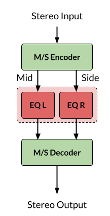
Unsurprisingly, after measuring different systems and comparing the results, I had to correct the topology of the processing chain (the initial version was introduced in the Part I). The updated diagram is presented below, and the explanations follow it:

Compared to the original version, there are now 4 parallel input "lanes" (on the diagram, I have grouped them in 2x2 formation), and their function and the set of plugins comprising them is also different. Obviously, the most important component—the direct sound is still there, and similarly to the original version of the chain, the direct sound remains practically unaltered, except for adjusting the level of the phantom "center" compared to pure left and right and ambient components. By the way, instead of Mid/Side plugin I switched to "Phantom Center" plugin by Bertom Audio. The second lane is intended to control the level and the spectral shape of the ambient component.

Let me explain this frontend part before we proceed to the rest of the chain. After making the "spatial analysis" measurements, I realized that in a real speaker setup, the ambient component of the recording is greatly amplified by the room, and depending on the properties of the walls, it can even exceed in level "direct" signal sources. On measurements, this can be seen by comparing the magnitudes of uncorrelated (L→L, R→R), correlated (L+R→L, L+R→R), and anti-correlated (L-R→L, L-R→R) sets. The human body also plays an important role as an acoustical element here, and the results of measurements done using binaural microphones differ drastically from "traditional" measurements using a measurement microphone on a stand.

As a result, the ambient component has received a dedicated processing lane, so that its level and the spectral shape can be adjusted individually. By the way, in the old version of the chain, I used the Mid/Side representation of the stereo signal in order to tune the ambient sound component independently of the direct component. In the updated version, I switched to a plugin which extracts the phantom center based on the inter-channel correlation. As a result, pure unilateral signals are separated from the phantom center (recall from my post on Mid/Side Equalization that the "Mid" component still contains left and right, albeit in a reduced level compared to the phantom center).

Continuing on the chain topology, the output from the input lanes is mixed and is fed to the block which applies Mid/Side Equalization. This block replaces the FF/DF block I was using previously. To recap, the old FF/DF block was tuned after the paper by D. Hammershøi and H. Møller, which provides statistically averaged free-field and diffuse-field curves from binaural measurements of noise loudness on human subjects, compared to traditional noise measurements with a standalone microphone. The new version of the equalization block in my chain is derived from actual acoustic measurement in my room, on my body. Thus, I believe, it represents my personal characteristics more faithfully.

Following the Direct/Ambient EQ block, there are two parallel lanes for simulating binaural leakage and reproducing the effect of the torso reflection. This is part of the crossfeed unit, yet it's a bit more advanced than a simple crossfeed. In order to be truer to human anatomy, I added a delayed signal which mimics the effect of the torso reflection. Inevitably, this creates a comb filter, however this simulated reflection provides a significant effect of externalization, and also makes the timbre of the reproduced signal more natural. With careful tuning, the psychoacoustic perception of the comb filter can be minimized.

I must say, previously I misunderstood the secondary peak in the ETC which I observed when applying the crossfeed with the RedLine Monitor while having the "distance" parameter set to a non-zero value. Now I see that it is there to simulate the torso reflection. However, the weak point of such a generalized simulation is that the comb filter created with this reflection can be easily heard. In order to hide it, we need to adjust the parameters of the reflected impulse: the delay, the level, and the frequency response to match more naturally the properties of our body. After this adjustment, the hearing system starts naturally "ignoring" it, effectively transforming it into a perception of "externalization," same as it happens with the reflection from our physical torso. Part of adjustment that makes this simulated reflection more natural is making it asymmetric. Obviously, our physical torso and the resulting reflection is asymmetric as well.

Note that the delayed paths are intentionally band-limited to simulate partial absorption of higher frequencies of the audible range by parts of our bodies. This also inhibits the effects of comb filtering on the higher frequencies.

The output from the "ipsi-" and "contralateral" blocks of the chain gets shaped by crossfeed filters. If you recall, previously I came up with a crossfeed implementation which uses close to linear phase filters. I still use the all-pass component in the new chain, for creating the group delay, however, the shape of the magnitude response of the filter for the opposite (contralateral) ear is now more complex, and reflects the effect of the head diffraction.

And finally, we get to the block which adjusts the output to particular headphones being used. For my experiments and for recreational listening I ended up using Zero:Red IEMs by Truthear due to their low distortion (see the measurements by Amir from ASR) and "natural" frequency response. Yet, it is not "natural" enough for binaural playback, and still need to be adjusted.

Tuning the Processing Chain

Naturally, there are lots of parameters in this chain, and tuning it can be a time-consuming, yet captivating process. The initial part of tuning can be done objectively, by performing the "spatial signal analysis" mentioned before and comparing the results between different setups. It's unlikely that any of the setups is "ideal," and thus the results need to be considered with caution and shouldn't be just copied blindly.

Another reason why blind copying is not advised is due to uncertainties of the measurement process. From the high level point of view, a measurement of the room sound via binaural microphones blocking the ear canal should be equivalent to the sound that arrives to ear-blocking IEMs by wires. Conceptually, IEMs will just propagate the sound further, to the ear drum. The problem is that a combination of arbitrary mics and arbitrary IEMs create a non-flat "insertion gain." I could easily check that by making a binaural recording and then listening to it via IEMs—it's "close," but still not fully realistic. Ideally, a headset with mics should be used which was tuned by the manufacturer to achieve a flat insertion gain. However, in practice it's very hard to find a good one.

Direct and Ambient Sound Field Ratios

Initially, I've spent some time trying to bring the ratios between correlated and uncorrelated components, and the major features of their magnitude response differences to be similar to my room setup. However, I was aware that the room has too many reflections, and too much uncorrelated sound resulting from it. This is why the reproduction of "off-stage" positions from the test track described in the part II of the blog post series has some technical flaws. Nevertheless, let's take a look at these ratios. The graph below shows how the magnitude response of fully correlated (L+R) components differ from uncorrelated direct paths (L→L, R→R), averaged, and smoothed psychoacoustically (as a reminder, this is a binaural measurement using microphones that block the ear canal):

We can see that the bass sums up and becomes louder than individual left and right channels by 6 dB—that's totally unsurprising because I have a mono subwoofer, and the radiation pattern of LXmini speakers which I used for this measurement is omnidirectional at low frequencies. As the direction pattern becomes more dipole-like, the sound level of the sum becomes closer to the sound level of an individual speaker. Around 2 kHz the sum even becomes quieter than a single channel—I guess this is due to acoustical effects of the head and torso. However, the general trend is what one would expect—two speakers play louder than one.

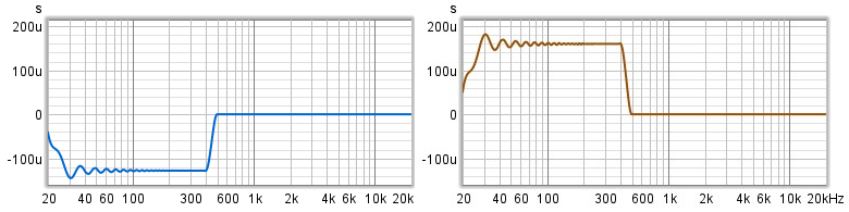
Now let's take a look at the magnitude ratio between the anti-correlated, "ambient" component, and fully correlated sound. Basically, the graph below shows the magnitude response of the filter that would turn the direct sound component into the ambient component:

It's interesting that in theory, anti-correlated signals should totally cancel each other. However, that only happens under ideal conditions, like digital or electrical summing—and that's exactly what we see below 120 Hz due to the digital summing of the signals sent to the subwoofer. But then, as the signal switches to stereo speakers, there is far less correlation, and cancellation does not occur. In fact, due to reflections and head refraction, these initially anti-correlated (at the electrical level) signals become more correlated, and can even end up having higher energy than correlated signal, when summed. Again, we see that around the 2 kHz region, and then, around 6.5 kHz, and 11 kHz.

The domination of the ambient component can actually be verified by listening. To confirm it, I used my narrow-banded mono signals, and created an "anti-correlated" set by inverting the right channel. Then I started playing through speakers pairs of correlated and anti-correlated test signals for the same frequency band—and indeed—sometimes the anti-correlated pair sounded louder! However, the question is—should I actually replicate this behavior in the headphone setup, or not?

The dominance of the ambient (diffuse) component over direct (free-field) component around 6.5 kHz and 11 kHz agrees with the diffuse-field and free-field compensation curves from the Hammershøi and Møller paper I mentioned above. However, in the 2 kHz region it's the free field component that should dominate.

I tried to verify whether fixing the dominance of the ambient component in the 1200—3000 Hz band actually helps to fix the issue with "off-stage" positions, but I couldn't! Trying to correct this band both with Mid/Side equalization, and with the "phantom center" plugin couldn't affect the balance of fields, neither objectively (I re-measured with the same binaural approach), nor subjectively. I have concluded that either there must be some "destructive interference" happening to correlated signals, similar to room modes, or it's a natural consequence of head and torso reflections.

This is why subjective evaluations are needed. For comparison, this is how the balances between correlated and unilateral, and anti-correlated vs. correlated end up looking like in my headphone spatializer, overlaid with the previous graphs measured binaurally in the room, this is the direct component over unilateral signals:

This is the ambient component over direct:

Obviously, they do not look the same as their room-measured peers. The only similar feature is the peak in the diffuse component around 11 kHz (and I had to exaggerate it to achieve the desired effect).

You might have noticed two interesting differences: first, the level of the fully correlated sound for the spatializer is not much higher than levels of individual left and right channels. Otherwise, the center sounds too loud and close. Perhaps, this has something to do with a difference how binaural summing works in the case of dichotic (headphone) playback versus real speakers.

The second difference is in the level of bass for the ambient component. As I've found, enhancing the level of bass somehow makes the sound more "enveloping." This might be similar to the difference between using a mono subwoofer vs. stereo subwoofers in a room setup, as documented by Dr. Griesinger in his AES paper "Reproducing Low Frequency Spaciousness and Envelopment in Listening Rooms".

The other two "large-scale" parameters resulting from the spatial signal analysis that I needed to tune were the magnitude profile for the contra-lateral ear (the crossfeed filter), and the level of reverb. Let's start with the crossfeed filter which is linked to shoulder reflection simulation.

Shoulder Reflection Tuning And Crossfeed

The shoulder reflection I mentioned previously quite seriously affects the magnitude profile for all signals. Thus, if we intend to model the major peaks of valleys of the magnitude profile for the crossfeed filter, we need to take care of tuning the model of the shoulder reflection first. I start it objectively, by looking at the peaks in the ETC of the binaural recording. We are interested in the peaks that are located at approximately 500–700 microsecond delay—this is the approximate distance from the shoulder to the ear. Why not to use the exact distance measured on your body? Since we are not modeling this reflection faithfully, it will not sound natural anyway. So we can start from any close enough value and then adjust by ear.

There are other reflections, too: the closest to the main pulse are reflections from the ear pinna, and further down in time are wall reflections—we don't model these. The reason is that wall reflections are confusing, and in the room setup we usually try to get rid of them. And pinna reflections are so close to the main impulse, so they mostly affect the magnitude profile, which we adjust anyway.

So, above is the ETC graph of direct (ipsilateral) paths for the left ear. Contralateral paths are important, too (also for the left ear):

Torso reflections have rather complex pattern which heavily depends on the relative position of the source to the body (see the paper "Some Effects of the Torso on Head-Related Transfer Functions" by O. Kirkeby et al as an example). Since we don't know the actual positions of virtual sources in stereo encoding, we can only provide some ballpark estimation.

So, I started with an estimation from these ETC graphs. However, in order to achieve more naturally sounding setup, I've turned to listening. A reflection like this usually produces a combing effect. We hear this combing all the time, however we don't notice it because the hearing system tunes it out. Try listening to a loud noise, like a jet engine sound, or sea waves—they sound "normal." However, if you change your normal torso reflection by holding a palm of a hand near your shoulder, you will start hearing the combing effect. Similarly, when the model of the torso reflection is not natural, combing effect can be heard when listening to correlated or anti-correlated pink noise. The task it to tweak the timing and relative level of the reflection to make it as unnoticeable as possible (without reducing the reflection level too much, of course). This is what I ended up with, overlaid with the previous graphs:

Again, we can see that they end up being different from the measured results. One interesting point is that they have to be asymmetrical for left and the right ear, as this leads to more naturally sounding result.

Reverberation Level

Tuning the reverberation has ended up being an interesting process. If you recall previous posts, I use actual reverberation of my room, which sounds surprisingly good in the spatializer. However, in order to stay within the reverb profile recommended for music studios, I reduce its level to make it decay faster than in real room. Adding too much reverb can be deceiving because it makes the sound "bigger" and might improve externalization, however it also makes virtual sources too wide and diffuse. This of course depends on the kind of music you are listening to, and personal taste.

There are two tricks I've learning while experimenting. The first one I actually borrowed from Apple's spatializer. While analyzing their sound, I've found that they do not apply reverb below 120 Hz, like, at all. Perhaps, this is done to avoid effects of room modes. I tried that, and it somewhat cleared up the image. However, having no bass reverb makes the sound in headphones more "flat." I decided to add the bass back, but with a sufficient delay, in order to minimize its effect. I also limited it application to "ambient" components only. As a result, the simulated sound field has become wider and more natural. Below are reverb levels for my room, my processing chain, and for comparison purpose, captured from Apple's stereo spatializer, playing through AirPods Pro.

The tolerance corridor is calculated for the size of the room that I have.

We can see that for my spatializer, the reverb level is within the studio standard. And below is the Apple's reverb:

A great advantage of having your own processing chain is that you can experiment a lot, something that is not really possible in a physical room and with off-the-shelf implementations.

Tuning the Headphones

As I've mentioned, I found Zero:Red by Truthear to be surprisingly good for listening to the spatializer. I'm not sure whether this is due to their low distortion, or due to their factory tuning. Nevertheless, the tuning has still to be corrected.

Actually, before doing any tuning, I had to work on the comfort. These Zero:Reds have quite a thick nozzle—larger than 6 mm in diameter, and with any stock ear tips they were hurting my ear canals. I found tips with thinner ends—SpinFit CP155. With them, I almost forget that I have anything insert into my ears.

Then, the first thing to tune was to reduce the bass. Ideally, the sensory system should not be able to detect that the sound is originating from the source close to your head. For that, there must be no vibration perceived. For these Zero:Reds I had to reduce overall bass region by 15 dB down, plus address individual resonances. A good way to detect them is to run a really long logarithmic sweep through the bass region. You would think that reducing the bass that much makes the sound too "lightweight," however, the bass from reverb and late reverb does the trick. In fact, one interesting feeling that I get is the sense of floor "rumbling" through my feet! Seriously, first couple of times I was checking if I accidentally left the subwoofer on, or is it vibration from the washing machine—but in fact this just is a sensory illusion. My hypothesis is that there are perception paths that help to hear the bass by feeling it with body, and these paths are at least partially bidirectional, so hearing the bass in headphones "the right way" somehow can invoke a physical feeling of it.

All subsequent tuning was more subtle and subjective, based on listening to many tracks and correcting what wasn't sounding "right." That's of course not the best way to do tuning, but it worked for me on these particular IEMs. After doing the tweaking, I have compared the magnitude response of my spatializer over Zero:Reds with Apple's spatializer over AirPods. In order to be able to compare "apples to apples," I have measured both headphones using the QuantAsylum QA490 rig. Below is how the setup looked like (note that on the photo, I have ER4SRs inserted into QA490, not Zero:Reds):

And here are the measurements. Note that since QA490 is not an IEC-compliant ear simulator, measured responses can only be compared to each other. The upper two graphs are for the left earphone, the lower two are for the right headphone, offset by -15 dB. Measurements actually look rather similar. AirPods can be distinguished by having more bass, and I think that's one of the reasons why to my ears they sound less "immersive" to me:

Another likely reason is that I tend to use linear phase equalizers, at the cost of latency, while Apple spatializer likely uses minimum phase filters which modify timing relationships severely.

Conclusion

Creating a compelling, and especially "believable" stereo spatialization is anything but easy. Thankfully, these days even at home it is possible to make measurements that may serve as a starting point for further adjustment of the processing chain. A challenging part is finding headphones that would allow disappearing in one's ears, or on one's head, as concealing them from the hearing system is one of the prerequesites for tricking the brain that the sound is coming from around you.

Friday, September 22, 2023

(Almost) Linear Phase Crossfeed

After checking how Mid/Side EQ affects unilateral signals (see the post), I realized that a regular minimum phase implementation of crossfeed affects signals processed with Mid/Side EQ in a way which degrades their time accuracy. I decided to fix that.

As a demonstration, let's take a look at what happens when we take a signal which exists in the left channel only and first process it with crossfeed, and then with a Mid/Side EQ filter. Our source signal is a simple Dirac pulse, attenuated by -6 dB. Since we apply digital filters only, we don't have to use more complicated measurement techniques that involve sweeps or noise. The crossfeed implementation is my usual Redline Monitor plugin by 112 dB, with the "classical" setting of 60 degrees virtual speaker angle, zero distance and no center attenuation. Then, a Mid/Side linear phase (phase-preserving) EQ applies a dip of -3 dB at 4.5 kHz with Q factor 4 to the "Mid" component only. Below I show in succession how the frequency and phase response, as well as the group delay of the signal changes for the left and the right channel.

This is the source signal:

This is what happens after we apply crossfeed. We can see that both amplitude and phase got modified, and the filter intentionally creates a group delay in order to imitate the effect of a sound wave first hitting the closer ear (this is what I call the "direct" path), and then propagating to more distant one, on the opposite side of the head (see my old post about the Redline Monitor plugin), I call this the "opposite" path:

And now, we apply Mid/Side EQ on top of it (recall that it's a dip of -3 dB at 4.5 kHz with Q factor 4 to the "Mid" component only):

Take a closer look at the right channel, especially at the group delay graph (bottom right). You can see a wiggle there which is on the order of the group delay that was applied by the crossfeed filter. Although the amplitude is down by about -22 dB at that point, this is still something we can hear, and this affects our perception of the source position, making it "fuzzier."

As I explained previously in the post on Mid/Side Equalization, changing the "Mid" and the "Side" components independently makes some artifacts being produced when we combine the M/S components in order to convert them back into L/R stereo representation. Application of the crossfeed prior to the Mid/Side equalization adds a huge impact both to the phase and to the group delay. This is because a minimum phase implementation of the crossfeed effect creates different phase shifts for the signals on the "direct" and on the "opposite" paths. To demonstrate that it's indeed due to the phase shifts from the crossfeed, let's see what happens when we instead use linear phase filters in the crossfeed section (the shape of the magnitude response is intentionally not the same as of the Redline):

This looks much better and clean. And as you can see, the filter still modifies the group delay and phase, but not across the whole spectrum. That's why I call this implementation "Almost Linear Phase." What we do here is we still apply a frequency-dependent delay to the signal, however we do it more surgically, only in the region where we do not expect any modifications done by the Mid-Side EQ part. That means, both the linear phase crossfeed and the M/S EQ filters must be developed and used together. That's exactly what I do in my evolving spatializer implementation (see Part I and Part II). As I know that in my chain the M/S equalization is only applied starting from 500 Hz (to remind you, it is used to apply diffuse-to-free field (and vice versa) compensation separately to correlated and negatively correlated parts of the signal), I developed a crossfeed filter which only applies the group delay up to that frequency point, and keeping the phase shift at 0 afterwards.

Note that 500 Hz does not actually correspond to physical properties of sound waves related to the human head size. In typical crossfeed implementations, the delay for imitating sound wave propagation is applied up to 700–1100 Hz (see publications by S. Linkwitz and J. Conover). Thus, limiting the application to lower frequencies is sort of a trade-off. However, if you recall the "philosophy" behind my approach—that we don't actually try to emulate speakers and the room, but rather try to extract the information about the recorded venue, with minimal modifications to the source signal, this trade-off makes sense.

Crossfeed Filter Modeling

One possible approach I could use to shape my crossfeed filters is to copy them from an existing implementation. However, since with linear phase filters I can control the amplitude and the phase components independently, I decided to read a bit more recent publications about head transfer function modeling. I found two excellent publications by E. Benjamin and P. Brown from Dolby Laboratories: An Experimental Verification of Localization in Two-Channel Stereo and The effect of head diffraction on stereo localization in the mid-frequency range. They explore the effect of the frequency-dependent changes of the acoustic signal as it reaches our ears, which happens due to diffraction of the sound by the head. I took these results into consideration when shaping the filter response for the opposite ear path, and also when choosing the values for the group delay.

Besides the virtual speakers angle, Redline Monitor also has the parameter called "center attenuation." This is essentially the attenuation of the Mid component in the Mid/Side representation. Thus, the same effect can be achieved by putting the MSED plugin (I covered it in the post about Mid/Side Equalization) in front of the crossfeed, and tuning the "Mid Mute" knob to the desired value (it is convenient that MSED actually uses decibels for "Mid Mute" and "Side Mute" knobs).

As for the "distance" parameter of Redline Monitor, I don't intent to use it at all. In my chain, I simulate the effect of distance with reverb. In Redline Monitor, when one sets the "distance" to anything other than 0 m, the plugin adds a combing filter. Another effect that the "distance" parameter affects is the relative level between the "direct" and the "opposite" processing paths. This makes sense, as the source which is closer to the head will be more affected by the head shadowing effect than the source far away. In fact, the aforementioned AES papers suggest that by setting ILD to high values, for example 30 dB, it is possible to create an effect of a talker being close to one of your ears (do you recall Dolby Atmos demos now?). However, since I actually want headphone sound to be perceived further from the head, I want to keep the inter-channel separation as low as possible, unless it degrades lateral positioning.

Filter Construction

I must note that constructing an all-phase filter with a precisely specified group delay is not a trivial task. I have tried many approaches doing this "by hand" in Acourate, and ended up with using Matlab. Since it's a somewhat math-intensive topic, I will explain it in more details in a separate post. For now, let's look again at the shapes for the group delay of such a filter, for the "direct" path and the "opposite" path:

This is the filter which delays the frequencies up to 500 Hz by 160 μs (microseconds). After the constant group delay part, it quickly goes down to exactly zero, also bringing back the phase shift to 0 degrees. That's how we enable the rest of the filter to be phase preserving. Those who a bit familiar with signal processing could ask—since a constant positive group delay means that the phase shift is linearly going down, where did it start from a non-zero value in the first place? The natural restriction on any filter is that at 0 Hz frequency (sometimes this is called the "DC component") it must have either 0 or 180 degrees phase shift. What we do in order to fulfill this requirement, is we use the region from 0 to 20 Hz to build up the phase shift rapidly, and then we bring it down along the region from 20 Hz to 500 Hz (note that the frequency axis start from 2 Hz on the graphs below):

Yes, the group delay in the "ultrasound" region is a couple of milliseconds, which is an order of magnitude greater than the group delay used for crossfeed. But, since we don't hear that, it's OK.

A delaying all-pass filter is used for the "opposite" path of the crossfeed filter. For the "direct" path, we need to create an inverse filter in terms of the time delay, that means, a filter which "hastens" the group delay. This is to ensure that a mono signal (equal in the left and right channels) does not get altered significantly by our processing. Such a signal is processed by both the "direct" and the "opposite" filters, and the results are summed. If the delays in these filters are inverse of each other, the sum will have a zero group delay, otherwise it won't.

The similar constraint is applied to the frequency response. That means, if we sum the filters for the "direct" and the "opposite" channels, the resulting frequency response must be flat. This is also true for the original minimum-phase Redline filters.

So, I used the following steps in order to produce my linear phase versions of crossfeed filters using Acourate:

  1. With help of Matlab, I have created an all-pass filter which applies a 160 µs delay between 20 and 500 Hz, and a filter which speeds up the same region by 128 µs (the reason for inexact symmetry is that the channel on the "opposite" path is attenuating). The important constraint is that the resulting group delay between paths must be between about 250–300 µs.

  2. I created a simple sloped down amplitude response: starting from -3.3 dB at 20 Hz and ending with -9 dB at 25600 Hz, and with help from Acourate convolved it with the delaying all-pass filter—this has become the starting point for the "opposite" path filter. For the direct path, I simply took the "direct" path filter which has the needed "anti-delay" (hastening), and a flat magnitude response.

Then I applied the following steps multiple times:

  1. Sum filters for the "direct" and the "opposite" paths. The resulting amplitude will not be flat, and now our goal is to fix that.

  2. Create an inverse frequency response filter for the sum (Acourate creates it with a linear phase).

  3. Convolve this inverse filter with either the filter for the "direct" or for the "opposite" path. This is a bit of an art—choosing the section of the filter to correct, and which path to apply it to. The aim is to retain a simple shape for both paths of the filter.

Below are the shapes I ended up with:

The filters that we have created can be cut to 16384 taps for the 96 kHz sampling rate. We need to keep relatively large number of taps in order to have enough resolution at low frequencies where we perform our phase manipulations.

Is There Any Difference?

After going through all these laborious steps, what improvements did we achieve over the original minimum phase filters of the Redline Monitor? First, as I've mentioned in the beginning, the main goal for me was to eliminate any phase difference between left and right channels after crossfeed processing in order to minimize artifacts from Mid/Side EQing. As we have seen in the first section of the post, this goal was achieved.

Sonically, a lot of difference can be heard even when listening to pink noise. Below is a recording where I switch between unprocessed pink noise combined from a correlated layer and an anti-correlated layer, then processed using RedLine Monitor at 60 degrees, 0 m distance, 0 dB center, and then processed with my almost linear-phase crossfeed (the track is for headphone listening, obviousl):

To me, my processing sounds more like how I hear the unprocessed version on speakers (the actual effect heavily depends on the headphones used). The noise processed by Redline has fuzzier phantom center, and there is much less enveloping on the sides. So I think, the (almost) linear phase implementation of crossfeed is sonically more accurate.

Monday, July 10, 2023

Headphone Stereo Setup Improved, Part II

In the Part I of these post series, I presented the architecture of my headphone audio processing chain along with an overview of the research it is based upon. In the Part II (this post), I'm presenting test tracks that I use in the process of adjusting the parameters, and the framework and tools for understanding them. The description of the adjustment process thus slips to upcoming Part III of this series of posts.

A Simplified Binaural Model of Hearing

Before we dive into tracks, I would like to explain my understanding of binaural hearing mechanism by presenting a simple model that I keep in my mind. Binaural hearing a very complex subject and I'm not even trying to get to the bottom of it. I have compiled together information from the following sources:

Note that the models presented in these sources are different from one another, and as it usually happens in the world of scientific research, there can be strong disagreements between authors on some points. Nevertheless, there is a number of aspects on which most of them agree, and here is what I could distill down:

From my understanding, after performing auto-correlation and per-band stabilization of auditory images for the signals in each ear, the brain attempts to match the information received from the left and the right ear in order to extract correlated information. Discovered inter-aural discrepancies in time and level allow the auditory system to estimate the position of the source, using learned HRTF data sets. Note that even for the same person there can be multiple sets of HRTFs. There is an understanding that there exist "near-field" and "far-field" HRTFs which can help in determining the distance to the source (see this AES paper for an example).

For any sound source for which the inter-aural correlation is not positive, there are two options:

  • If the sound has an envelope (that is, a period of onset and then a decay), its position will likely be "reset" to "inside the head." This applies both to uncorrelated and anti-correlated sounds. I'm not sure about the reason of the "resetting" for anti-correlated signals, however for uncorrelated signals this is pretty obvious as no remote external sound source can produce unilateral audio images. So the brain decided that the source of the sound must be a bug near your ear, or maybe even inside it :)

  • If the sound lacks an envelope: a continuous noise or buzz for example, it can remain "outside the head," however it's position will not be determined. In the real world, I did encounter such cases in airport and shops, when a "secured" door left open somewhere far away is making continuous ringing or beeping, and the sound is kind of "floating" around in the air, unless you get youself close enough to the source of the signal so that the inter-aural level difference can help in localizing it.

An important takeaway from this is that there are many parameters in the binaural signal that must be "right" in order for the hearing system to perceive it as "natural."

The Goniometer Tool

For me, the best tool for exploring properties of the correlation between the channels of a stereo signal is the goniometer. In its simplest form, it's a two-dimensional display which shows the combined output from the left and the right channels, in time domain. Basically, it visualizes the mid-side representation which I was discussing in the previous post. Usually the display is graded in the following way:

Even this simplest implementation can already be useful in checking whether the signal is "leaning" towards left or right, or perhaps there is too much uncorrelated signal. Below are renderings of stereo pink noise "steered" into various spatial directions. I have created these pictures based on views provided by the JS: Goniometer plugin bundled with the Reaper DAW):

The upper row is easy to understand, the interesting thing though is that while purely correlated or purely anti-correlated noise produces a nice line—that's because samples in both channels always carry either exactly the same or strictly opposite values, the mix of correlated and anti-correlated noise sort of "blows up" and turns into a fluffy cloud. Also, when panning purely correlated or anti-correlated noise, it just rotates around the center. Whereas, panning of the mix of correlated and anti-correlated looks like we are "squeezing" the cloud until it becomes really thin. Finally, with initially correlated signal, adding a small delay in one channel destroys correlation of higher frequencies, and what used to be a thin line becomes a cloud squeezed from the sides.

To see the latter effect in more detail, we can use a more sophisticated goniometer implementation which also shows the decomposition in the frequency domain, in addition to the time domain. For example, I use the free GonioMeter plugin by ToneBoosters. Below is the view on the same signal as in the bottom right corner of the previous picture:

The time-domain goniometer display is at the center—the same squeezed cloud, and to the left and to the right of it we can see a frequency-domain view of correlation and panning. This is the tool which I used to get an insight into the techniques used for stereo imaging of my test tracks.

Test Tracks

Now, finally, let's get to the tracks and how I use them. Overall, these tracks serve the same purpose as test images for adjusting visual focus in optical equipment. The important part about some of them is that I know which particular effect the author / producer wanted to achieve, because it's explained either in the track itself, or in the liner notes, or was explained by the producer in some interview. With regular musical tracks we often don't know whether what we hear is the "artistic intent" or merely an artefact of our reproduction system. Modern producer / consumer technology chains like Dolby Atmos are intended to reduce this uncertainty, however for traditional stereo records there are lots of assumptions that may or may not hold for the reproduction system being used, especially for headphones.

Left-Right Imaging Test

This is Track 10 "Introduction and Left-Right Imaging Test" from "Chesky Records Jazz Sampler & Audiophile Test Compact Disc, Vol. 1". This track is interesting because apart from conventional "between the speakers" positions, it also contains "extreme left" ("off-stage left") and "extreme right" positions that span beyond speakers. This effect is achieved by adding anti-correlated signal to the opposite channel. Let's use the aforementioned GonioMeter plugin for that. This is the "center" position:

Midway between center and right:

Fully to the right, we can see that the inter-channel correlation across the frequency range is dropping to near zero or lower:

Off-stage right, channels have entered the anti-correlated state, note that the panning indicator at the top part of the time-domain view does not "understand" the psychouacoustic effect of this:

And for comparison, here is off-stage left—similarly anti-correlated channels, however the energy is now on the left side:

Considering the "extreme" / "off-stage" positions, we can see that although the stereo signal is panned to the corresponding side, the opposite channel is populated with anti-correlated signal. Needless to say, the "off-stage" positions do not work with headphones unless some stereo to binaural processing is applied. The brain is unable to match the signals received from the left and the right ear, and "resets" the source position to "inside the head." Binaural processing adds necessary leaking thus allowing the brain to find similarities between the signals from the left and the right ears and derive the position.

Following the binaural model I have presented in the beginning of the post, the "extreme" left and right positions from the "Left-Right Imaging Test" can't be matched to a source outside of the head unless we "leak" some of that signal into the opposite ear, to imitate what happens when listening over speakers. However, if the room where the speakers are set up is too "live," these "off-stage" positions actually end up collapsing to "inside the head"! Also, adding too much reverb may make these extreme positions sounding too close to "normal" left and right positions, or even push them between the positions of virtual speakers.

That's why I'm considering this track to be an excellent tool not only for testing binarual rendering, but also for discovering and fixing room acoustics issues.

Natural Stereo Imaging

This is Track 28 "Natural Stereo Imaging" from "Chesky Records Jazz Sampler & Audiophile Test Compact Disc, Vol. 3" (another excellent sampler and a set of test recordings). The useful part in this track is the live recording of a tom-tom drum naturally panned around the listener. I have checked how the "behind the listener" image is produced, and found that it also uses highly decorellated stereo. This is "in front of the listener" (center):

And this is "behind the listener":

We can see that level-wise, they are the same, however the "behind the listener" is has negative inter-channel correlation. Needless to say, correct reproduction of this recording over the headphones requires cross-feed. But there is another thing to pay attention to. As the drum is moving around the listener, in a natural setting I would expect the image to stay at the same height. In headphones, this requires both correct equalization of the frontal and diffuse components, and some level of added reverberation in order to enrich the diffuse component with high frequencies. If the tuning isn't natural, the auditory image of the drum may start changing its perceived height while moving to sides and behind the head, for example, it might suddenly start appearing significantly lower than when it was in the front of the head.

Get Your Filthy Hands Off My Desert

This is track 7 or 8, depending on the edition, of Pink Floyd's "The Final Cut" album. The track is called "Get Your Filthy Hands Off My Desert" and contains a spectacular effect of a missile launched behind the head and exploding above the listener. The perceived height of the explosion helps to judge the balance between "dark" and "bright" tuning of the headphones.

Another good feature of the track is the spaciousness. As I understand it, the producer was using the famous Lexicon 224 reverberation unit (a brainchild of Dr. David Griesinger) in order to build the sense of being in the middle of a desert.

The Truths For Sale (the ending)

This is the final 1/2 minute of the Track 4 from "Judas Christ" album by gothic metal band Tiamat. For some reason it's not a track on its own, but it really could be. I must say that I listen to this album since it was released in 2002, but never until I started digging into headphones tuning this fragment really stood out for me. It was a pleasant shock when I've realized how much externalized and enveloping can it sound. Similar to the Brian Eno's music (see below), it's very easy to believe that the droning sound of the track is really happening around you.

Being part of a metal album, this track contains a lot of bass. Perhaps, too much. It's a good test to see whether the particular headphones are too heavy on the bass side. In this case, their resonances seriously diminish the sense of externalization because, thanks to the sensation of vibration, your brain realizes that the source of the sound is on your head. That's why this track complements well the previous one when checking the balance between low and high frequencies.

Spanish Harlem

Track 12 from the album "The Raven" by Rebecca Pidgeon is an audiophile staple. It's the famous "Spanish Harlem" track, it presents acoustically recorded ensemble of instruments and a female vocal. I use it for checking "apparent source width" and also localization of the instruments when comparing between different processing tunings.

The producer of this record, Bob Katz, recommends checking for bass resonances by listening to loudness of individual bass notes in the beginning of the track. Although, his advice was addressing subwoofer tuning, it applies to headphones as well, as they can also have resonances. Luckily, bass unevenness is much less concerning with headphones.

Ambient 1: Music For Airports

This is Track 1 from "Ambient 1: Music For Airports" by Brian Eno. It doesn't have a real title, just a mark that it's track 1 on the side 1 of the original vinyl issue of this album. This is an ambient track with sound sources floating around and lots of reverb, another very good example of the power of the Lexicon 224 reverb unit.

For me, this track is special because with a more or less natural headphone tuning it allows me to get into a state of transcending inside the world built by the sound of the album. My brain starts to perceive the recorded sounds as real ones, and I get a feeling that I don't have any headphones in/on my ears. I think, this happens because the sounds are somewhat "abstract" and it makes it easier for the brain to believe that they actually can exist around me in the room. Also, the sources are moving around, and this helps the brain to build up a "modified" HRTF for this particular case.

It's interesting, that after "priming" the auditory system with this track, all other tracks listened in the same session also sound very natural. I can easily distinguish between tracks with a good natural spaciousness, and tracks that resemble "audio cartoons," in the sense that they lack any coherent three-dimensional structure. I suppose, this state is that's the highest level of "aural awareness" which usually requires a room with a controlled reverb, and a very "resolving" speaker system. I'm glad that I can achieve that with just headphones.

Immaterial

I could easily use the entire album "Mine" by Architect (a project of Daniel Myer, also known for the Haujobb project) for the purpose of testing source placement and envelopment. This electronic album is made with a solid technical knowledge about sound and understanding of a good spectral balance, and is a pleasure to listen to. However, I don't actually listen to this track myself during the tuning process. Instead, I render the track 5, Immaterial via the processing chain after completing the tuning in order to catch any clipping that may occur due to extra gain resulting from equalization. Below are the short-term and overall spectral views of the track:

We can see that the track has a frequency profile which is actually more similar to white noise, not pink noise, thus it features a lot of high frequency content, that is, a lot of "air." That means, if I tilt the spectrum of the processing chain in favor of high frequencies, with this track there is a higher chance to encounter clipping. The sound material on this album also uses quite massive synthesized bass. That's why it's a good track to validate that the gain of the processing chain is right across the entire spectrum.

Synthetic and Specially Processed Signals

I could actually list much more tracks that I briefly use for checking this or that aspect of tuning, but we have to stop at some point.

While "musical" recordings are useful for checking general aspects of the tuning, in order to peek into details, we can use specially crafted sounds that represent a specific frequency band, for example. Traditionally, such sounds are obtained from synthesizers or noise generators, however I've found that processed "real" sounds tend to provide more stable results when judging the virtual source position.

In my process, I use recordings of percussion instruments: tambourine, bongos, and the snare drum. By themselves, they tend to occupy a certain subset of the audio spectrum, as we can see on the frequency response graph below (the snare drum is the green line, bongos are the red line, tambourine is the blue line):

However, to make them even more "surgical," I process them with a linear phase notch filter and extract the required band. This of course makes the resulting sound very different from the original instrument, however it preserves the envelope of the signal, and thus the ability of the brain to identify it. I use the critical bands of the Bark scale, as it has strong roots in psychoacoustics.

I took these instrument recordings from an old test CD called Sound Check, produced in 1993 by Alan Parsons and Stephen Court. The CD contains a lot of good uncompressed and minimally edited recordings, and for me, it stands together with the demo/test CDs from Chesky Records.

Consumer Spatializers

So, I'm going this DIY path, however these days there exist very affordable spatializers built into desktop and mobile OSes that can do binaural playback for stereo, and even employ head tracking, after "magically" guessing your HRTF from photographs of your head and ears. For sure, I did try these, however consumer-grade spatializers do not perform well on all my test tracks. For example, the "off-stage" positions from Left-Right Imaging Test we not rendered correctly by any spatializer I tried, instead it was collapsing to inside the head. The closest to my expectation was the Apple spatializer for AirPods Pro in the "head tracking" mode, however even in this case more or less correct positioning was observed for the right "off-stage" position only.

Yet another problem with consumer-grade spatializers I tried is that for lower latency they tend to use minimum-phase filters, and these distort the phase and group delay while applying signal magnitude equalization. This essentially kills the perception of the performance space which I preserve with my processing chain where I always use linear-phase filters. Each time I tried to substitute an LP filter with an MP equivalent (in terms of signal magnitude), the reproduction was blurred down and degrading into essentially a two-dimensional representation.

If I have a budget for that, I would go with a "proper" binaural spatializer like Smyth Realizer. But I don't, and for me making my own spatializer is the only viable alternative to get the sound I want.

Conclusions

It's a really long road to getting to a natural reproduction of stereo records in headphones, and we are slowly making it. In the process of making anything well, good tools are of a paramount importance. I hope that the description of the goniometer, and its application to analysis of described test tracks, as well as their intended use, did help. A lot more material will be covered in subsequent posts.

Sunday, June 4, 2023

On Mid/Side Equalization

After finishing my last post on the headphone DSP chain, I intended to write the second part which should provide examples of adjusting the parameters of the chain effects for particular models of headphones. However, while writing it I had encountered some curious behavior of the mid/side equalization module, and decided to figure out what's going on there and write about it.

Let's recall last part of the DSP chain that I have proposed previously. Note that I've changed the order of the effects application, I will explain the reason at the end of the post:

The highlighted part is the pair of filters which apply diffuse field to free field (df-to-ff) or vice versa (ff-to-df) correction EQ curves to mid and side components separately. To remind you, these are intended to help the brain to disambiguate between "in front of the head" and "behind the head" audio source positions, with a goal to improve externalization. As I've found, well made headphones likely only need just one of the corrections applied. For example, if the headphones are tuned closer to the "diffuse field" target, then they already should reproduce "behind the head" and "around you" sources realistically, however, frontal sources could be localized "inside the head." For such headphones, applying a df-to-ff compensation to the "mid" component helps to "pull out" frontal sources from inside the head and put them in the front. Conversely, for the headphones tuned with a preference for the "free field," it's beneficial to apply "ff-to-df" correction to the side component of the M/S representation in order to make surrounding and "behind the head" sources to be placed correctly in the auditory image.

Now, a discovery which was surprising for me was that the application of a mid/side equalization affects reproduction of unilateral (existing in one channel only) signals. A test signal sent to the left channel exclusively, was creating a signal in the right channel as a result of passing through the mid/side equalizer. And that's even with all cross-feeding turned off, of course. This had caught me by surprise because I knew that converting between stereo and mid/side representations should be lossless and that also assumes that no signals appear out of nowhere. So, what's going on here?

The Sinusoids Algebra

What I have realized is that all this behavior appears to be surprising at first only because addition and subtractions of audio signals is in fact not very intuitive. In order to get a good grasp of it, I went through Chapter 4 of Bob MacCarthy's book "Sound Systems: Design and Optimization". It provides a very extensive and insightful coverage with just a minimal help of math. I think, it's worth stating here some facts from it about summing of two sinusoidal signals of the same frequency:

  1. When adding signals of different amplitudes, it's the amplitude of the loudest signal, and the difference between amplitudes that matter the most. The phase of the weaker signal is of a lesser significance. There is a formula to express this fact: Sum = 20*Log10((A + B) / A) (A is the level of the louder signal). Graphically the resulting levels for in-phase signals summation look like this:

  2. Only when adding or subtracting signals that have similar amplitudes their relative phase (we can also say the "phase shift") starts to matter.

  3. There is no linear symmetry between the case when the two added signals of the same amplitude are in phase, and the case when they are completely out of phase. In the first case the amplitude doubles, whereas in the second case they fully cancel each other out. People who ever tried building their own loudspeakers are well aware of this fact. This is the graphical representation of the resulting amplitude depending on the phase shift:

Another thing worth understanding is how the inter channel correlation coefficient (ICCC) depends on the relationship between the signals. This is the "correlation" gauge which we observe in plugins dealing with M/S manipulations. What plugins typically show is the correlation at the "zero lag," that is, when there is no extra time shift between the signals (in addition to the shift they already have).

As a side note, a lot of times the calculation of cross-correlation is carried out in order to find how much one signal needs to be shifted against another in time in order to achieve the maximum match. That's why "lag" is considered. By the way, here is a nice interactive visualization of this process by Jack Schaedler. However, for the purpose of calculating the ICCC we only consider the case of non-shifted signals, thus the "lag" is 0.

In the case of zero lag, the correlation can be calculated simply as a dot product of two signals expressed as complex exponentials: A(t)*B̅(t), where denotes a complex conjugate of B. Since we deal with the same signal, and its version shifted in phase, the parameters for the frequency mutually cancel each other, and what we left with is just the cosine of the phase shift. That should be intuitively clear: for signals in phase, that is, with no phase shift, the ICCC is cos(0)=1.0, for signals completely out of phase (phase shift π/2) the correlation is cos(π/2)=0, and finally, when the first signal is phase inverted compared to the second one, the ICCC is cos(π)=-1.0.

By the way, since we deal with a "normalized" correlation, that is, having the value between -1.0 and 1.0, the ICCC does not depend on the relative amplitude of the signals. Thus, for example, in-phase signals of the same amplitude have the same ICCC as in-phase signals with a relative level of -60 dB. Strictly speaking, when there is no signal with matching frequency in another channel, their correlation is not defined, however, for simplicity plugins show the ICCC of 0 in this case.

ICCC and Mid/Side Signal Placement

From the previous fact, it can be seen that ICCC actually does not fully "predict" how a pair of signals in the left and the right channel will end up being placed in the Mid/Side representation. That's because ICCC only reflects their phase shift, while the result of summation also depends on their relative levels. For a better understanding of relationship between the stereo and M/S representations we need a two-dimensional factor, and the visual representation of this factor is what the tool called "goniometer" shows. I will use it when talking about my test signals and tracks in the next post.

To round up what we have just understood, let's consider the process of making the M/S representation of an input stereo signal. If we consider each frequency separately, then we can apply the facts stated above to each pair of individual sinusoids from the left and the right channel. This adds more details to a somewhat simplistic description I provided in the previous post.

If the sinusoid in one of the channels is much higher in the amplitude than in another channel, then both summation and subtraction will produce a signal which is very similar to the stronger source signal, and the weaker signal will only make a small contribution to the result, regardless of its relative phase.

That means, a strong unilateral signal will end up being both in the "mid" and the "side" components, minimally affected by the signal of the same frequency from the opposite stereo channel. Note that if we normalize the resulting amplitudes of the "Mid" and "Side" signals by dividing them by 2, we will actually see a signal of a lower amplitude there. Here is an illustration—an example stereo signal is on the top, it has the level of the right channel lower by -12 dB. The resulting "Mid Only" and "Side Only" versions are below it:

In the case when there is no signal of this frequency in the opposite channel, then exactly the same signal will land both into both M/S components, with the amplitude divided by 2. This is the picture from the previous post showing that for the two sinusoids in the middle of the top picture:

If both channels of the input stereo signal contain the signal of a particular frequency with close enough amplitudes, then the outcome depends on the relative phase between these signals. As we know, in the "extreme" cases of fully correlated or fully anti-correlated signals, only the mid or the side component will end up carrying this frequency (this was also shown on a picture in the previous post). For all the cases of the phase lying in between, the result will get spread out between the mid and the side, below is an example for the case of a 140 deg phase offset (ICCC=-0.766) which results in a -12.6 dB reduction of the original signal level as a result of summation:

Note that the resulting sinusoids in the mid and the side channels have a phase shift from the signal in the left channel which is different both from what the signal in the right channel has, and from each other.

Since the process of decoding the stereo signal from the M/S representation is also done via addition and subtraction, the same sinusoids algebra applies to it as well.

What If We Change Just Mid or Side?

It's interesting that despite the fact that separate mid/side equalization is an old technique used by both mixing and mastering engineers, thanks to its benefits for the ear, it's side effects on the signal are not described as widely. However, if you read the previous section carefully, you now understand that making level and phase adjustments to the mid or to the side components only will inevitably affect the outcome of "decoding" the M/S representation back into stereo.

For simplicity, let's focus on amplitude changes only. Making changes both in amplitude and phase will cause even more complex effects when the signals get summed or subtracted. That means, we apply a "linear phase" equalizer. We can use either an equalizer which provides mid/side equalization directly, for example: the "LP10" plugin by DDMF, or "thEQorange" by MAAT digital. However, in fact, we can use any linear phase equalizer which provides two independently controlled channels because we can wrap it between two instances of the MSED plugin: the first one needs to "encode" stereo into the M/S representation, and the second one will produce the stereo version back from the modified signal, as shown below:

(even though MSED is completely free, if you want an alternative for some reason, there is also the "Midside Matrix" plugin by Goodhertz, also free).

Since no equalizer can affect just a single frequency only, instead of looking at sinusoiods in the time domain as we will switch into the frequency domain. My approach to testing here is to use the same log sweep in the both channels, and modify either amplitude of relative phase of the second channel, as we did before. Then I capture what comes out in the left and the right channel after an EQ applied separately to the Mid or the Side representation.

I start with the case which had initially drawn my attention: a unilateral stereo signal (in the left channel only) for which we apply some equalization to the mid component. Let's see what do left and right channels contain after we apply a simple +10 dB, Q 5 gain to the 920 Hz center frequency to the mid component only:

As you can see, indeed after this equalization a signal has appeared in the right channel! Another interesting observation is that the level of the gain for the unilateral signal is actually less than +10 dB. That's because the gain that we have applied to the mid component was combined with the unmodified (flat) signal from the side component. Only in the case when there was no side component at all—identical signals in the left and the right stereo channels—the equalization of the mid component will look like a regular stereo equalization. Certainly, it is good to be aware of that!

By the way, I tried both LP10 and thEQOrange and their behavior is the same. Considering that LP10 costs just about $40, and thEQOrange almost 15 times more, it's good to know that you can get away with a cheaper option unless you strongly prefer the UI of thEQOrange.

Now, I was genuinely interested in seeing what my FF-to-DF and DF-to-FF Mid/Side equalization do to unilateral signals. Here are some examples comparing the effect on the fully correlated signal (shades of green) with the signal induced in the opposite channel for a unilateral input:

We can see that in some cases the levels of signals induced in the opposite channel are significant and can be only -15 dB lower than the "main" signal. However, we need to recall that the FF/DF compensation comes after we have applied the cross-feed unit. That means, we never really have unilateral stereo signals. To check what actually happens, I put the "direct" path processing in front of the FF/DF unit and used the same initially unilateral test signals. This is what I've got:

These curves definitely look less frightening. Thanks to crossfeed, any unilateral signal penetrates into the opposite channel.

Conslusions

What have we learned from this lengthy exploration? First, it's soothed my worries about the side effects of the Mid/Side equalization. Since I only use it with much more correlated signals than the edge case of a unilateral stereo signal, the side effects are not as significant, while the win of the FF/DF compensation is audibly perceivable.

Second, looking closer at what happens during the M/S equalization helped me to reveal and fix two issues with my initial chain topology:

  1. I reordered the units in the output chain, putting the FF/DF unit before the L/R band alignment unit. That's because I have realized that individual equalization of the left and the right channels inevitably affects the contents of the mid/side representation. For example, a signal which initially was identical between the left and the right channels will obviously lose this property after going through an equalizer which applies different curves to the left and the right channels.

  2. Since for the FF/DF I actually use the MConvolutionEZ plugin—with a linear phase filter—I noticed that the approach of applying the convolution to the mid and side components recommended in the manual does not work well for my case. What MeldaProduction recommends is to chain two instances of MConvolutionEZ: one in "Mid" mode and one in "Side" mode one after another. This in fact creates a comb filter because mid and side are now processed with a one sample delay, and then get summed (I did confirm that). So instead of doing that, I wrapped MConvolutionEZ between two instances of MSED (as I've shown above) and just use it in the regular "stereo" mode. This ensures that both mid and side are processed with no time difference.

I also considered, if it's possible to create a Mid/Side equalization which avoids processing of sufficiently uncorrelated signals in order to avoid the side effects described above. A search for "correlation-dependent band gain change" led me to a bunch of microphone beamforming techniques. Indeed, in beamforming we want to boost the frequency bands that contain correlated signals, and diminish uncorrelated signals (noise). However, thinking about this a bit more, I realized that such processing becomes dependent on the signal, and thus isn't linear anymore. As we saw previously with my analysis of the approaches for automatic gain control such signal-dependent processing can add significant levels of non-linear distortion. That's probably why even sufficiently expensive mastering equalizers don't try to fight the side effects of mid/side equalization.