In a recent post titled "(Almost) Linear Phase Crossfeed" I only explained my intents for creating these filters and the effect I achieved with them. In this post I'll explain the underlying math and go through the MATLAB implementation.
I called this post "The Math of The ITD Filter" for the reason I think this naming is more correct. This is because the purpose of this all-pass filter is just to create an interaural time delay (ITD). Thus, it's not a complete cross-feed or HRTF filter but rather a part of it. As mentioned in the paper "Modeling the direction-continuous time-of-arrival in head-related transfer functions" by H. Ziegelwanger and P. Majdak, an HRTF can be decomposed into three components: minimum phase, frequency-dependent TOA (time-of-arrival), and excess phase. As authors explain, the "TOA component" is just another name for the ITD psychoacoustic cue, and that is what our filters emulate.
Time-Domain vs. Frequency-Domain Filter Construction
Since there is a duality between time and frequency domains, any filter or a signal can be constructed in one of them and transformed into another domain as needed. The choice of the domain is a matter of convenience and of the application area. If you are looking for concrete examples, there is an interesting discussion in the paper "Transfer-Function Measurement with Sweeps" by S. Müller and P. Massarani about time-domain and frequency-domain approaches for generation of log sweeps used in measurements.
Constructing in the time domain looks more intuitive at the first glance. After all, we are creating a frequency dependent time delay. So, in my initial attempts I experimented with splitting the frequency spectrum into bands using linear phase crossover filters, then delaying these bands, and combining them back. This is an easy and intuitive way for creating frequency-dependent delays, however stitching these differently delayed bands back does not happen seamlessly. Because of abrupt changes of the phase at connection points, the group delay behaves quite erratically. I realized that I need to learn how to create smooth transitions.
So my next idea was to create the filter by emulating its effect on a measurement sweep, and then deriving the filter from this sweep. This is easy to model because we just need to delay parts of the sweep that correspond to affected frequencies. Since in a measurement sweep each frequency has its own time position, we know which parts we need to delay. "To delay" in this context actually means "alter the phase." For example, if the 1000 Hz band has to be delayed by 100 μs, we need to delay the phase of that part of the sweep by 0.1 * 2π radians. That's because a full cycle of 1 kHz is 1 ms = 1000 μs, so we need to hold it back by 1/10 of the cycle.
This phase delay can be created easily while we are generating a measurement sweep in the time domain. Since we "drive" this generation, we can control the delay and make it changing smoothly along the transition frequency bands. I experimented with this approach, and realized that manipulation of the phase has its own constraints—I have explained these in my previous post about this filter. That is, for any filter used for real-valued signals, we have to make to phase to start from 0 at 0 Hz (DC), and end with zero phase at the end of our frequency interval (half of the sampling rate). The only other possibility is to start with π radians and end with π—this creates a phase-inverting filter.
This is how this requirement affects our filter. Since we want to achieve a group delay which is a constant over some frequency range, it implies that the phase shift must change with the constant rate on that range (this is by the definition of the group delay). That means, the phase must be constantly decreasing or increasing, depending on the sign of the group delay. But this descent (or ascent) must start somewhere! Due to the restriction I stated in the previous paragraph, we can't have a non-zero phase at 0 Hz. So, I came to an understanding that I need to build a phase shift in the ultrasound region, and then drive the phase back to 0 across the frequency region where I need to create the desired group delay. Phase must change smoothly, as otherwise its derivative, the group delay, will jump up and down.
This realization finally helped me to create the filter with the required group delay behavior. However, constructing the filter via the time domain creates artifacts at the ends of the frequency spectrum (this is explained in the paper on measurements sweeps). Because of that, modern measurement software usually uses sweeps generated in the frequency domain. These sweeps are also more natural for performing manipulations in the frequency domain, which can be done fast by means of direct or inverse FFTs. So, after discussing this topic on the Acourate forum, I've got advice from its author Dr. Brüggemann to construct my filters in the frequency domain.
Implementation Details
Creating a filter in the frequency domain essentially means generating a sequence of complex numbers corresponding to each frequency bin. Since we generate an all-pass filter, the magnitude component is always a unity (zero amplification), and we only need to generate values to create phase shifts. However, the parameters of the filter we are creating are not phase shifts themselves but rather their derivatives, that is, group delays.
This is not a big problem, though, because mostly our group delay is a constant, thus it's a derivative of a linear function. The difficult part is to create a smooth transition of the phase between regions. As I have understood from my time-domain generation attempts, a good function for creating smooth transitions is the sine (or cosine), because its derivative is the cosine (or sine) which is essentially the same function, but phase-shifted. Thus, the transitions of both the phase and the group delay will behave similarly.
So, I ended up with two functions. The first function is:
φ_main(x) = -gd * x
And its negated derivative is our group delay:
gd = -φ_main'(x)
The "main" function is used for the "main" interval where the group delay is the specified constant. And another function is:
φ_knee(x) = -gd * sin(x)
Where gd is the desired group delay in microseconds. By choosing the input range we can get an ascending slope which transitions into a linear region, or a descending slope.
Besides the group delay, another input parameter is the stop frequency for the time shift. There are also a couple of "implicit" parameters of the filter:
- the band for building the initial phase shift in the ultrasound region;
- the width of the transition band from the time shift to zero phase at the stop frequency.
Graphically, we can represent the phase function and the resulting group delay as follows (the phase is in blue and the group delay is in red):

Unfortunately, the scale of the group delay values is quite large. Here is a zoom in on the region of our primary interest:

For the initial ramp up region, I have found that a function sin(x) + x gives a smoother "top" compared to a sine used alone. So there is the third function:
φ_ramp(x) = (sin(x) +x) / π
Note that this function does not depend on the group delay. What we need from it is to create the initial ramp up of the phase from 0 to the point where it starts descending.
Getting from the phase function to the filter is rather easy. The complex number in this case is e iφ. The angle φ is in radians, thus the values produced by our φ_main and φ_knee, must be multiplied by 2π.
Since we work with discrete signals, we need to choose how many bins of the FFT to use. I use 65536 bins for the initial generation, this has enough resolution in the low frequency region. And the final filters can be made shorter by applying a window (more details are in the MATLAB section below).
Verification in Audio Analyzers
Checking the resulting group delay of the filter is possible in the MATLAB itself, as I have shown in the graphs above. However, to double-check, we want to make an independent verification using some audio analyzing software like Acourate or REW. For that, we need to apply inverse FFT to the FFT we have created, and save the resulting impulse response as a WAV file. Below is a screenshot from FuzzMeasure (I used it because it can put these neat labels on the graph):

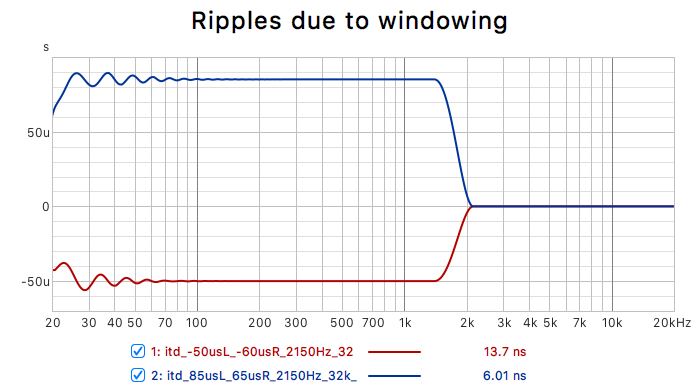
I loaded two impulses, both ending at 2150 Hz: one has a -50 μs group delay (red graph), another 85 μs (blue graph). The absolute values of the group delay displayed on the graph (170+ ms) are not important because they are counted from the beginning of the time domain representation, thus they depend on the position of the IR peak. What we are interested in are the differences. We can see that at the flat region past 2 kHz the value is 170.667 ms for both graphs. Whereas, for the blue graph the value at ~200 Hz is 170.752 ms. The difference between these values is 85 μs. For the red graph, the difference is 617-667 = -50 μs. As we can see, this agrees with the filter specification.
In REW, the group delay is relative to the IR peak. However, it has a different issue. Being a room acoustics software, REW by default applies an asymmetric window which significantly truncates the left part of the impulse. This works great for minimum-phase IRs, however since the IR of our filter is symmetric, this default weighting creates as significant ripple at low frequencies:
In order to display our filter correctly, we need to choose the Rectangular window in the "IR windows" dialog, and expand it to maximum both on the left and the right side:

After adjusting windowing this way, the group delay is displayed correctly:

We can see that the group delays are the same as before: -50 μs and 85 μs. Thus, verification confirms that the filters do what is intended, but we need to understand how to use audio analyzing software correctly.
MATLAB Implementation Explained
Now, knowing that our filter works, let's understand how it is made. The full code of the MATLAB script is here, along with a couple of example generated filters.
The main part is the function called create_itd_filter.
This is its signature:
function lp_pulse_td = create_itd_filter(...
    in_N, in_Fs, in_stopband, in_kneeband, in_gd, in_wN)
The input parameters are:
in_N: the number of FFT bins used for filter creation;in_FS: the sampling rate;in_stopband: the frequency at which the group delay must return to0;in_kneeband: the frequency at which the group delay starts its return to0;in_gd: the group delay for the "head shadowing" region;in_wN: the number of samples in the generated IR after windowing.
From these parameters, the script derives some more values:
    bin_w = in_Fs / in_N;
    bin_i = round([1 18 25 in_kneeband in_stopband] ./ bin_w);
    bin_i(1) = 1;
    f_hz = bin_i .* bin_w;
bin_w is the FFT bin width, in Hz. Using it, we
calculate the indexes of FFT bins for the frequencies we are interested
in. Let's recall the shape of our group delay curve:

Note that 1 Hz value is only nominal. In fact, we are
interested the first bin for our first point, so we set its index
explicitly, in order to avoid rounding errors. And then we translate bin
indexes back to frequencies (f_hz) by multiplying them by
the bin width. Use of frequencies that represent the centers of bins is
the usual practice for avoiding energy spillage between bins.
Next, we define the functions for the phase, either directly, or as integrals of the group delay function:
    gd_w = @(x) -in_gd * x; % f_hz(3)..f_hz(4)
    syms x;
    gd_knee_f = -in_gd * (cos(pi*((x - f_hz(4))/(f_hz(5)-f_hz(4)))) + 1)/2;
    gd_knee_w = int(gd_knee_f);
    gd_rev_knee_f = -in_gd * cos(pi/2*((x - f_hz(3))/(f_hz(3)-f_hz(2))));
    gd_rev_knee_w = int(gd_rev_knee_f);
gd_w is the φ_main function from the
previous section. It is used between the frequency points
3 and 4. gd_knee_f is the
knee for the group delay, its integral is the φ_knee
function for the phase shift. As a reminder, this knee function is used
as a transition between the constant group delay (point
4) and zero delay (point 5). We run
the cosine on the interval [0, π], and transform it, so
that it yields values in the range from 1 to
0, allowing us to descent from in_gd to
0.
But we also need to have a knee before our constant group delay (from the point 2 to the point 3), to ramp it up from 0. Ramping up can be done faster, so we run the cosine function on the interval [-π/2, 0]. The resulting range goes naturally from 0 to 1, no need to transform it.
Now we use these functions to go backwards from the point 5 to the point 2:
    w = zeros(1, in_N);
    w(bin_i(4):bin_i(5)) = subs(gd_knee_w, x, ...
        linspace(f_hz(4), f_hz(5), bin_i(5)-bin_i(4)+1)) - ...
        subs(gd_knee_w, x, f_hz(5));
    offset_4 = w(bin_i(4));
    w(bin_i(3):bin_i(4)) = gd_w(...
        linspace(f_hz(3), f_hz(4), bin_i(4)-bin_i(3)+1)) - ...
        gd_w(f_hz(4)) + offset_4;
    offset_3 = w(bin_i(3));
    w(bin_i(2):bin_i(3)) = subs(gd_rev_knee_w, x, ...
        linspace(f_hz(2), f_hz(3), bin_i(3)-bin_i(2)+1)) - ...
        subs(gd_rev_knee_w, x, f_hz(3)) + offset_3;
    offset_2 = w(bin_i(2));
Since gd_knee_w and gd_rev_knee_w are
symbolic functions, we apply them via the MATLAB function
subs. When going from point to point, we need to move each
segment of the resulting phase vertically to align the connection
points.
Now, the interesting part. We are at the point 2,
and our group delay is 0. However, the phase shift is
not 0, you can check the value of offset_2
in the debugger if you wish. Since the interval from the point
1 to the point 2 lies in the
ultrasonic region, the group delay there is irrelevant. What is
important is to drive the phase shift so that it is equal to
0 in the point 1. This is where the
φ_ramp function comes handy. It has a smooth top which
connects nicely to the top of the knee, and it yields 0
at the input value 0.
    ramp_w = @(x) (x + sin(x)) / pi;
    w(bin_i(1):bin_i(2)) = offset_2 * ramp_w(linspace(0, pi, bin_i(2)-bin_i(1)+1));
Then we fill our the values of FFT bins by providing our calculated phase to the complex exponential:
pulse_fd = exp(1i * 2*pi * w);Then, in order to produce a real-valued filter, the FFT must be symmetric relative to the center frequency (see this summary by J. O. Smith, for example). So, for example, the FFT (Bode plot) of the filter may look like this:

Below is the code that performs necessary mirroring:
    pulse_fd(in_N/2+2:in_N) = conj(flip(pulse_fd(2:in_N/2)));
    pulse_fd(1) = 1;
    pulse_fd(in_N/2+1) = 1;
Now we switch to the time domain using inverse FFT:
pulse_td = ifft(pulse_fd);This impulse has its peak in the beginning. In order to produce a linear phase filter, the impulse must be shifted to the center of the filter:
lp_pulse_td = circshift(pulse_td, in_N/2-pidx+1);And finally, we apply the window. I used REW to check which one works best, and I found that the classic von Hann window does the job. Here we cut and window:
    cut_i = (in_N - in_wN) / 2;
    lp_pulse_td = lp_pulse_td(cut_i:cut_i+in_wN-1);
    lp_pulse_td = hann(in_wN)' .* lp_pulse_td;
That's it. Now we can save the produced IR into a stereo WAV file. I use a two channel file because I have found that having a bit of asymmetry works better for externalization:
lp_pulse_td1 = create_itd_filter(N, Fs, stopband, kneeband, gd1, wN);
lp_pulse_td2 = create_itd_filter(N, Fs, stopband, kneeband, gd2, wN);
filename = sprintf('itd_%dusL_%dusR_%dHz_%dk_%d.wav', ...
    fix(gd1 * 1e6), fix(gd2 * 1e6), stopband, wN / 1024, Fs / 1000);
audiowrite(filename, [lp_pulse_td1(:), lp_pulse_td2(:)], Fs, 'BitsPerSample', 64);
These IR files can be used in any convolution engine. They are also can be loaded into audio analyzer software.
Application and Thoughts on Asymmetry
For a practical use, we need to create 4 filters: a pair for ipsi- and contra-lateral source, and these are different for the left and right ear. Why the asymmetry? The paper I referenced in the introduction of this post, and other papers suggest that ITD of real humans are not symmetrical. My own experiments with using different delay values also confirm that asymmetric delays feel more natural. It's interesting that even the delay of arrival between ipsi- and contra-lateral ears can be made slightly different for the left and right direction. Maybe this originates from the fact that we never hold our head ideally straight. The difference is quite small anyway. Below are the delays that I ended up using for myself:
- ipsilateral left: -50 μs, right: -60 μs;
- contralateral left: 85 μs, right: 65 μs.
As we can see, difference between the left hand source path and the right hand source path is 10 μs (135 μs vs. 125 μs). This corresponds approximately to a 3.4 mm sound path, which seems to be reasonable.
Note that if we take the "standard" inter-ear distance of 17.5 cm, that gives us roughly a 510 μs TOA delay. However, this corresponds to a source which is 90° from the center. While, for stereo records we should use just about one third of this value. Also, your actual inter-ear distance can be smaller. In any case, since this is just a rough model, it makes sense to experiment and try using different values.
Regarding the choice of the frequencies for the knee- and stop-bands. With the increase of the frequency the information from the phase difference becomes more and more ambiguous. Various sources suggest that the ambiguity in the time information starts at about 1400 Hz. My own brief experiments suggest that if we keep the ITD along the whole audio spectrum, it makes determination of source position more difficult for narrowband sources starting from 2150 Hz. Thus, I decided to set the transition band between those two values.