Saturday, December 18, 2021

YouTube Music and Intersample Peaks

A while ago I was checking how Google Play Music and the playback chain following it are handling intersample peaks. Since then, GPM was retired and replaced with YouTube Music (YTM), browsers got uncountable number of updates, and so on. Did the situation with digital headroom improve? I was stimulated to check this by the fact that I tried using YTM in Chrome browser on my Linux laptop, and was disappointed with the quality of the output. Before that, I was using YTM on other OSes, and it was sounding fine. Is there anything wrong with Linux? I decided to find out.

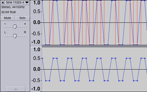
I have updated my set of test files. I took the same test signal I used back in 2017: a stereo file where both channels carry a sine at the quarter of the sampling rate (11025 or 12000 Hz), with a phase shift at 45 degrees. The left channel has this signal normalized to 0 dBFS, and this creates intersample overs peaking at about +3 dBFS, and the right channel has this signal at the half of the full scale (6 dB down), which provides enough headroom and should survive any transformations:

I have produced a set of test files to include all the combinations of the following attributes:

  • sample rate: 44.1 and 48 kHz;
  • bit width: 16 and 24;
  • dither: none and triangular.

There are two things that I can validate using these signals: non-linearities introduced by clipping or compression of intersample peaks, and whether the inter channel balance stays the same. For measuring non-linearities I used the THD+N measurement. Although, due to the fact that the signal is at the quarter of the sampling rate, even the second harmonic is out of frequency range, the "harmonic distortion" part of this measurement doesn't make much sense, however the "noise" part still does. There is a strong correlation between the look of the frequency response graph and the value of the THD+N.

I have uploaded my test signals to YouTube Music and then measured the THD+N in the following clients:

  • the official web client running in recent stable versions of Chrome and FireFox on Debian Linux, macOS, and Windows,
  • and the official mobile apps running on an Android phone (Pixel 5) and iPad Air.

All the outputs were measured using a digital capture chain. For macOS and Windows I used a hardware loopback on RME FireFace card. For Linux I used Douk Audio USB to S/P-DIF digital interface (Mini XMOS XU208) which was connected by optics to the FireFace card. For mobile devices I used a dual USB sound card iConnectAudio4 by iConnectivity. The sound cards were configured either at 44.1 or at 48 kHz.

Observations and Results

The first thing I've noted was that YouTube Music stores audio tracks at 44.1 kHz sample rate (this is confirmed by looking at the "Encoding Specifications" in the YT tech support pages), and 48 kHz files got mercilessly resampled, clipping the channel with overs quite severely. This can be easily seen by comparing the difference between the L&R channels of the signal played back—it's only 4.34 dB instead of 6 dB. Below is the spectrum of the 48 kHz test signal after it has went through YTM's server guts:

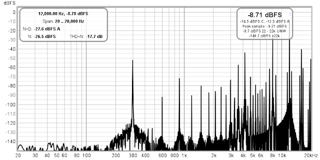
Also, it can be seen from the graph, YTM does some "loudness normalization" by scaling the amplitude of the track down, likely after resampling it to 44.1 kHz. This causes the peaks on both channels to be down by about 11 dB. Actually, that's good because it provides needed headroom for any sample rate conversions happening after the tracks leave the YTM client.

As for the lossy compression, it actually doesn't add much artifacts, as we can see from this example:

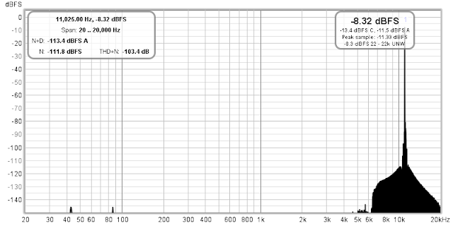
Yes, there is a "bulb" around the original signal likely added due to the fact that the codec works in the frequency domain and has reduced resolution. However, the THD+N of this signal is just 3 dB down (-103.4 dB) from the 16-bit dithered original (-106.8 dB), and it's still on par with capabilities of good analog electronics. So, lossy codec is not on the list of my concerns for the content on YTM.

Desktop Clients

On desktop, the difference in the measurements only depends on the browser. However, the trouble with Linux is that both Chrome and FireFox always switch the output to 48 kHz as they start playing even if the PulseAudio daemon is configured to use 44100 Hz for both the "default" and "alternative" sample rates. As we will see, this does a bad job for Chrome and likely was the reason why I felt initially that something is going wrong with YTM on Linux.

Yet another interesting observation on the desktop is that in case the browser does a bad job of resampling, bringing the digital volume control down on the YTM client does not provide any extra headroom for the browser's processing. That was a bummer! Apparently, the order of the processing blocks has changed, compared to Play Music, putting the digital attenuation after resampling, maybe because YTM uses some modern web audio API which gives the browser more control over media playback.

Here is a summary of THD+N measurements for Chrome and FireFox for cases when the system output is either at the "native" sampling rate—44.1 kHz or at 48 kHz. On the left there are baseline numbers for the original dithered signal, measures for the left and the right channel are delimited with a common slash:

Signal Chrome to 44 Chrome to 48 FireFox to 44 FireFox to 48
24/44, -146.7 / -139.2 -102.7 /-103.7 -29.6 / -82.6 -103.4 / -103.7 -103.3 / -103.5
16/44, -106.8 / -95.5 -102.9 / -97.8 -29.6 / -82.5 -102.1 / -97.8 -102.3 / -97.6
24/48, -147.5 / -139.7 -17.7 / -98.4 -17.7 / -80.6 -17.7 / -98.4 -17.7 / -98.4
16/48, -106.7 / -95.6 -17.7 / -89.4 -17.7 / -79.7 -17.7 / -89.5 -17.7 / -89.3

As we can see here, Chrome doesn't do a good job when it has to resample the output to 48 kHz, thus on Linux the only option is to use FireFox instead of it. And obviously, even FireFox can't undo the damage done to the original 48 kHz signal with intersample overs.

My guess would be that the audio path on FireFox uses floating point processing which creates necessary headroom, while Chrome still uses integer arithmetic.

Mobile Clients

Results from iOS are on par with FireFox confirming that this is likely the best result we can achieve with YTM. Android adds more noise:

Signal Android to 44 Android to 48 iOS to 44 iOS to 48
24/44, -146.7 / -139.2 -92.9 / -92.2 -92.9 / -92.2 -102.8 / -102.2 -102.8 / -102.2
16/44, -106.8 / -95.5 -92.6 / -88.3 -92.6 / -88 -101.8 / -97.7 -102 / -97.7
24/48, -147.5 / -139.7 -17.7 / -92 -17.7 / -92 -17.7 / -98.5 -17.7 / -98.5
16/48, -106.7 / -95.6 -17.7 / -87.9 -17.7 / -87.8 -17.7 / -89.4 -17.7 / -89.4

I had a chance to peek "under the hood" of Pixel 5 by looking at the debug dump of the audio service. What I could see there is that there are extra sample rate conversions happening on the way from the YTM app to the USB sound card. The app creates audio tracks with 44100 Hz sample rate. However, the USB audio on modern Android phones is managed by the same SoC audio DSP used for built-in audio devices, to bring down latency when using USB headsets. The DSP works at 48 kHz. Thus, even when the USB sound card is at 44.1, the audio tracks from YTM first got upsampled to 48 kHz to get to the DSP, and then DSP downsamples them back to 44.1 kHz for the sound card. I guess, on Apple devices either this pipeline is more streamlined, or everyone (including the DSP) use calculations providing enough headroom.

Conclusions

I think, it is all pretty clear, but here is the summary how to squeeze out the best quality from YouTube Music:

  • on desktop, when using Chrome (or Edge on Windows), set the sampling rate of the output to the native sample rate of YTM: 44.1 kHz, if that's not possible, use FireFox;
  • on Linux, always use FireFox instead of Chrome for running YTM client, because even lowering the digital volume on the YTM client does not prevent from clipping;
  • due to the fact that YTM applies volume normalization, there is no need to worry about having digital headroom on the DAC side;
  • any 48 kHz or higher content needs to be carefully resampled to 44.1 kHz before uploading to YTM to prevent damage from their sample rate conversion process.

Monday, November 1, 2021

Headphone Stereo Setup

After making a satisfying desktop stereo setup I decided to do something similar with headphones. As I had discussed before, right out of the box no headphones sound convincing to me simply due to physics and psychoacoustics issues that can't be solved using traditional headphone construction. As a result it's just not possible to reproduce a stereo record intended for speakers and expect having instruments placed correctly in the auditory image, even on "flagship" headphones. I'm always puzzled when I encounter phrases like "rock-solid imaging," in headphone reviews especially accompanied with measurement graphs confirming that the left and the right earphones are perfectly matched. I don't know—perhaps the reviewer has a perfectly symmetric head and body, and ideally matched ears—for my aging ears I know that the right one is about 3 dB more sensitive than the left one, so on perfectly matched headphone drivers I naturally have the auditory image shifted to the right slightly.

On the other hand, in order to achieve convincingly sounding stereo reproduction in headphones it's not necessary to go "full VR", measure individual HRTF of the listener in an anechoic chamber, and then perform physically correct simulation of speakers as virtual sound sources placed in front of the listener in a room, and moving around as the listener's head moves. In fact, after trying to use Waves NX for some time, I've found that head tracking only creates an additional distraction as it requires periodic resetting of the "neutral" head position due to headband shifting on the head. So I wanted something simpler, and I think I've found a good middle ground for myself with my setup.

In my headphone setup I follow the same principles as when setting up the desktop speakers—get the most important things right first, and then tune up the rest, getting as close to "ideal" as possible, but stopping when the cost of the next improvement becomes too high. However, the implementation of these principles is a bit different. There isn't as much of "physical alignment" in the headphone setup as one have to do for speakers. The only thing I had to ensure is that the headphone amplifier stays linear and doesn't produce distortions. Then most of the setup happens on the DSP side. But even there a distinction between "main" and "fine" tuning do exist.

As I had explained in my earlier post on headphone virtualization, reproduction over headphones lacks several components that we take for granted when listening over speakers:

  1. Room reverberation. This is a very important component which significantly supports the sound of the speakers themselves and also helps to place reproduced sources correctly in the auditory image. Acousticians love to talk about "direct-to-reverb" sound ratio when considering opera halls and other venues, as this is one of the parameters which separates good sounding spaces from bad sounding ones.

  2. Acoustical leakage between speakers. This is considered as a negative factor in VR over speakers applications, because for VR one needs to control precisely the sound being delivered to each ear, however stereo recordings actually rely on this acoustical leakage. Without it, sources that are hard panned to one channel tend to "stick" to the headphone which is playing them, narrowing the sound stage considerably.

  3. Assymetries in the human body and the hearing system. Listening over headphones makes the sounds coming into left and right ear very symmetric and this confuses the auditory system. Also, with aging, sensitivity of ears becomes less and less symmetrical, requiring individual tuning of headphones.

To achieve more realistic reproduction over headphones we need to replicate the effects of the factors listed above. Some manufacturers of headphones tried to do that in hardware, and we got products like AKG K1000 "earspeaker" headphones, which I guess sound almost right for stereo records, but are quite cumbersome to use, not mentioning the price. A good pair of open over-ear headphones can also come close to naturalistic stereo reproduction because they allow for some inter-aural leakage as well as slight interaction with the room. However, closed over-ear headphones and IEMs are hopeless in this respect, and only electronic or digital solutions can help them to produce a speaker-like stereo soundstage.

Before we dive into details of my setup, there are two main factors that are indicative for me when judging correctness of headphones tuning:

  • The sound is localized outside of the head. Although the actual perceived distance still depends on the recording, and sometimes it feels that the vocals are still very close to your face—for lots of modern records that's in fact the "artist's intention"—however, by quick A/B comparison with unprocessed headphone sounding one can quickly understand that although the sound appears to be close to the face, it's definitely not inside the head.

  • Every instrument can be heard distinctively, similar to how it sounds over well-tuned stereo speakers. By replicating the natural HRTF of the person via headphone tuning we "place" each frequency band correctly in the auditory image, and this allows the auditory system to separate auditory streams efficiently.

As a final analogy, putting on properly tuned headphones feels similar to wearing VR glasses—you feel "immersed" into scene, as if you are peeking into it via some "acoustic window."

The Tuning Process

The process of headphone tuning can be separated into several phases:

  1. Simulate ideal reverberation conditions for the actual room we are listening in. Although we can simply capture the reverb of the room, it's usually far from "ideal" due to strong reflections. If you went all the way building an ideal physical room—congratulations!—you can just use the captured response directly. However, one can just build a great virtual version of their room instead.

  2. Adjust the crossfeed and direct-to-reverb (D/R) ratio making sure that phantom sources end up placed correctly, especially those in "extreme" positions—outside the speakers. This tuning also moves the acoustic image out of the head.

  3. Tune the inter-aural frequency balance. This way we emulate the natural HRTF and any deficiencies of the individual's hearing apparatus that the brain got accustomed to.

  4. Finally, as an optional step we can use time domain signal correction to ensure that the electrical signal reaching the headphones has properties close to those of an ideal low-pass filter.

As for the headphones choice, my intention was to create tuning to use with Shure SRH-1540 closed-back headphones. These headphones are very comfortable to wear: lightweight, having a negligible pressure on the head, and not causing my ears to sweat. However, their factory tuning is too much V-shaped—a strange choice for "studio" headphones by the way. I strongly prefer the tuning of headphones made by Audeze because it resembles very close the sound of properly tuned speakers (and I have confirmed that by measuring with in-ear microphones), but the weight of magnetic planar headphones literally brings my head down (I made a comparison of the weights in one of my previous posts), and their thick faux leather pads quickly turn my ears into hot dumplings. So I ended up using Audeze EL-8 closed back as a tool for tuning, but after finishing with it I put them back into their box.

Reverberation

The idea behind replicating the reverberation of the room is that once we enter a room our hearing system adapts to it, and uses reflected sounds and reverberation as a source of information for locating positions of sources. This happens unconsciously—we just "feel" that the sound source is out there, without actually "hearing" the reflected sounds, unless the delay is large enough to perceive them as echoes. Thus, when we replicate the reverberation of the room over headphones, this helps the auditory system to perceive the sounds we hear as happening around us, in the room.

I captured the reverberation of my room using the classic technique of recording a pop of a balloon. Then I took the NX TrueVerb plugin and tried to tune the parameters so that resulting reverb matches the one I've captured. Speaking of "ideal" reverberation—I liked the idea of "ambechoic" room pioneered by G. Massenburg—I read about in the book "Acoustic Absorbers and Diffusers". The physical implementation of "ambechoic" requires using a lot of wide-band diffusers in order to "break up" all the reflections while retaining the energy of the reflected sound. In the virtual recreation, I simply turned off early reflections simulation and set the density of the emulated reverb tail to maximum value, and this is what I've got (ETC graph):

The first strong reflection (marked by the cursor) is created by the Redline Monitor, more on that later. Note that the reverb tail still looks a bit spiky, but this is the best I could obtain from TrueVerb.

I'm not very good at matching reverbs "by ear" so I used two tools: the IR measurements of Smaart V8 and the RT60 calculator of Acourate. The first has a good proprietary algorithm for finding the D/R ratio and overall decay times, the second shows in a convenient form decay times for each frequency band, and can display tolerance curves from standards.

Below are side by side comparisons of ETC for the real vs. emulated rooms as shown by Smaart V8:

I tried to get them as close as TrueVerb's controls allowed me to do. The early decay time (EDT) of the simulation is much shorted due to absence of early reflections, but I don't think it's an issue. The RT60 time is 25% shorter—I was trying to make it the same as of the room, however there are limits on the granularity of settings in TrueVerb. However, this shorter time is still good according to the comparison graph below—it shows per-frequency decay times along with tolerance boundaries from DIN 18041 standard for music reproduction calculated by Acourate for the room of my size:

Although I didn't try matching reverbs "by ear" I still listened to them carefully as measurements alone do not provide the full picture. During my early experiments I was intending to use the built-in reverb of my MOTU soundcard—after all it comes for free! However, despite looking similar on the measurement side, MOTU's reverb sounded horrible with very distinctive flutter echo. By the way, dry recordings of percussive musical instruments like castanets or bongos are turned out to be excellent for revealing any flaws in artificial reverbs.

Cross-feed and D/R ratio

TrueVerb was designed to be sufficient on its own for providing a stereo reverb and controlling its frequency response. However, the degree of control it provides wasn't enough for my specific needs. As a result, I ended up using the mono version of TrueVerb on two parallel buses, and augment it by Redline Monitor and an equalizer. Here is the connections diagram:

Note that TrueVerb outputs the reverb tail only. This way, I've got full control over the stereo dispersion and the spectral shape of the reverb tail. After playing with different settings on Redline Monitor I've ended up with 90 degree soundstage—this way, the reverb is sounding "enveloping", which was exactly my goal.

The direct sound is placed on a separate bus, with its own instance of Redline Monitor and own set of cross-feed parameters. By altering the volume control on this bus I can change the direct to reverb ratio.

On the Redline Monitor for the direct sound I've pinned the "speaker distance" parameter to the minimum value above zero: 0.1 meter. What I've found is that zero distance doesn't provide convincing externalization, however increasing of the speaker distance adds considerable combing effect, see my previous post about Redline Monitor for graphs. What I could see on the ETC graph is that enabling the "speaker distance" knob adds virtual reflections. Here I compare the settings of 0 meter distance, 0.1 meter, and 2.0 meter:

I suppose, the presence of reflections emulates the bounce of the sound from the mixing console (since Redline Monitor is intended for studios). As the "speaker distance" increases, the level of these reflections becomes higher compared to the direct impulse. That's understood—the further one moves away from the speakers, the more levels of the direct sound and the first reflection become similar. However, this increases the amplitude of comb filtering ripples, thus the minimum possible "speaker distance" is what we want to use. This settings keeps the emulated reflection at -26 dB, below the level of the direct sound—an acceptable condition if we consider a real acoustic environment.

After fixing the speaker distance I've spent some time tweaking multiple parameters which have turned out to be interconnected for the auditory system since changing one had effect on another:

  • the soundstage width,
  • the attenuation of the center channel (both parameters are on the Redline Monitor), and
  • relative levels between the direct sound bus and the reverb bus (D/R ratio).

While tweaking them I used stereo soundstage test tracks from Chesky Records demo CDs to ensure that sounds panned to left and right positions sound in headphones as if they are indeed coming from the corresponding speaker, and that "extreme" left and right—beyond the speakers—are reproduced convincingly. I also used music tracks with strong, energetic "in your face" mix (album "Cut" by the industrial "supergroup" C-Tec) to ensure that I could put the vocals further away from my face.

I tried to avoid attenuating the reverb too much compared to the direct sound as this dramatically decreases the perceived distance to the source. However, having the reverb too strong was breaking the perception of "extreme" left and right source positions, and so on. So finding the sweet spot for the combination of the simulation parameters turned out to be a challenging task and it actually gave me some intuitive understanding of how real speakers can interact with a real room.

Aligning Amplitude Response

Basically, what I have achieved through the previous stages is creating a virtual speaker setup in a virtual room with reverb similar to the one I have in my real room. Now I had to align the frequency response of that setup—as I hear it via the headphones—with the frequency response of my real speakers—as their sound reaches my ears. This process is often referred to as "headphones equalization." Traditionally it's done using a head and torso simulator, but I don't have one so I used in-ear microphones on my own head—that's even better because done this way the tuning becomes personal.

I used my Sennheiser Ambeo Headset for this task. I have captured the amplitude response of the speakers in Smaart V8 over the Ambeo sitting in my ears. Then I captured the amplitude response of EL-8s—also via Ambeo—and it has turned out to be quite close to speakers—no surprise that I like the sound of EL-8s so much. I must note that the positioning of centered banded noise was still wrong in EL-8 headphones. So even if I'd chosen to stick with them I still have to do some personal tuning, more about this later.

Nevertheless, what I wanted is to tune my SRH-1540s. I started measuring them, and they turned out to be way off the speaker sound "baseline": too much bass, and too much treble—the V-shape tuning in action. So I started equalizing them "in real time"—by adjusting the equalizer. I used a linear phase equalizer (LP10 by DDMF) to avoid altering the inter-aural time difference (ITD). This is because sharp EQ curves implemented using minimum phase filters can significantly affect the phase and thus change the ITD, since the tuning for the left and right ears is not symmetric.

After setting the amplitude response, I removed Ambeo from my ears—what a relief!—and performed final tuning strokes to make sure that all frequency bands are positioned consistently within the auditory image. This is extremely important in order to avoid spreading of auditory images of individual instruments.

For this step of tuning I used test signals generated by DGSonicFocus app by Dr. Griesinger. The app produces bands of noise centered between the channels. It can produce either correlated or decorrellated noise—I was using the latter option. When listening over correctly tuned speakers these test signal create a phantom center image. Thanks to my initial amplitude correction for headphone output, some of the bands were already placed correctly in the auditory image, but some still not, mostly in the high frequency range, because it's hard to tune high frequency region correctly from measurements only—they tend to be too volatile. So I used my ears instead, and by applying peaking EQs in the same linear phase equalizer managed to "move" all the bands to the center.

Below are the resulting EQ curves for SRH-1540. Note just how asymmetric they have to be in order to create a convincing auditory image for me over headphones:

I would compare this tuning process to making an individual pair of prescription glasses. Hopefully with advances in customer audio it will become much easier some day.

Time-Domain Tuning (optional)

Since I really enjoy what DSP filters produced by Acourate do to my speakers, I questioned myself whether it's worth to try applying Acourate to the headphone chain. After all, we are simulating speakers in a room so why not to try applying a room correction package to this simulation?

I did not plan doing acoustic measurements at the ear entrance as my equipment simply lacks the required precision. I decided to do the measurements at the analog electrical boundary by tapping into the headphone wires using my T-Cable. I temporarily bypassed the equalizer as it's linear phase, and its setting is asymmetric. From the measurements I've found that left and right outputs are almost identical, as I was expecting them to be on a proper audio chain. So, both the digital and the electrical analog chains are already almost perfect—is there really any room for improvement?

I ran Acourate's correction macros for these measurements, and it still managed to do something to the shape of the impulse response. Below is the difference, I think Acourate made it to look more like a minimum-phase response, notice the deeper "sagging" of the amplitude after the initial peak:

Did this correction change anything? Not too much in general, however percussion instruments started sounding a bit differently, and I would say towards more "natural" side. I loaded these corrections into a convolver plugin—adding it increased latency, but not significantly, since I already had the linear phase EQ plugin in the chain. Now I've got a feeling that I'm really done with the setup.

Putting it all Together

For completeness, here is the full processing chain I use for headphones tuning. I run it in Ardour together with the DSP filters for the speakers tuning:

Note that I marked how the sections of the chain conceptually relate to simulated speaker reproduction. As I noted previously, instead of multiple plugins for the "Room" part I could potentially use just one good reverb plugin, but I haven't yet found an affordable one which would fit my needs.

Despite using lots of plugins, the chain is not heavy on computations, and Ardour takes no more than 15% of CPU on my 2015 Mac mini (as measured by the Activity Monitor), leaving the fan being silent (and recall that Ardour also runs the speaker correction convolver).

Conclusions

Compared to setting up speakers, which was mostly done "by the book," setting up headphones required more experimenting and personal tweaking, but I think it was worth it. Would be interesting to do similar setup for IEMs, although doing measurements in this case for aligning with the speakers response will be challenging for sure.

About the time when I started doing these experiments, Apple has announced support for Atmos and binaural headphone rendering on headphones in their Music app. I took a try listening for some Atmos-remastered albums over headphones on an iPhone. The impression was close to what I have achieved for stereo recordings with my headphone setup—the same feeling of natural instrument placement, generally wider soundstage, and so on—definitely superior to a regular stereo playback over headphones. I was impressed that Apple and Dolby have achieved this effect over non-personalized headphones! On the other hand, expecting each album to be remastered in Atmos is unrealistic, so it's good I'm now able to listen to original stereo versions on headphones with the same feeling of "presence" that Apple provide in Atmos remasters.

Sunday, August 22, 2021

Automatic Gain Control

This post is based on the Chapter 11 of the awesome book "Human and Machine Hearing" by Richard Lyon. In this chapter Dr. Lyon goes deep into mathematical analysis of the properties of the Automatic Gain Control circuit. I took a more "practical" route instead, and did some experiments with a model I've built in MATLAB based on the theory from the book.

What Is Automatic Gain Control?

The family of Automatic Gain Control (AGC) circuits origins from radio receivers where it is needed to reduce the amplitude of the voltage received from the antenna in the case when the signal is too strong. In the old days the circuit used to be called "Automatic Volume Control" (A.V.C.), as we can see in the book on radio electronics design ("The Radiotron Designer's Handbook"):

However, the earliest AGC circuits can be found in the human sensory system—they help to achieve the high dynamic range of our hearing and vision. In the hearing system the cochlea provides the AGC function.

The goal of AGC is to maintain a stable output signal level despite variations in the input signal level. The stability of the output is achieved by creating a feedback loop which "looks" at the level of the output signal, and makes necessary adjustments to the input gain of the signal at the entrance to the circuit. This is how this can be represented schematically:

Note that the "level" is a somewhat abstract property of the signal. What we need to understand is that "level" can be tied, based on our choice, either to the amplitude of the signal or to it's power, and expressed either on a linear scale or on a logarithmic scale. There is also a somewhat arbitrary distinction between the "level" and the "fine temporal structure" of the signal. If we consider a speech signal, for example, it obviously has a high dynamic range due to fast attacks of consonant sounds. However, in AGC we don't examine the signal at such a "microscopic" level. There is always a time constant which defines the speed of level variations that we want to preserve in the output signal.

We want the gain changes to be bound to the "slow" structure of the output signal, otherwise we will introduce distortions. The AGC Loop Filter is used to express the distinction between "fast" and "slow" by applying smoothing the measured level. The simplest way of smoothing is applying a low-pass filter (LPF). Although it's common to define the LPF in terms of its cut-off frequency, another possible way is to use the "time constant", which defines the former.

AGC vs. Other Systems

There are two classes of systems that are similar to AGC in their function. The first class is comprised of systems controlled by feedback—these systems are studied extensively by the engineering discipline called "Control Theory". Schematically, a feedback-controlled system looks like this:

The big difference with AGC is that there is a "desired state" of the controlled system—this is what the control system is driving it towards. For example, in an HVAC system the reference is the temperature set by the user. In contrast, nobody sets the reference for an AGC circuit, instead, for any input signal that doesn't change for some time, the AGC circuit settles down on some corresponding output level which is referred to as "equillibrium."

Another class of systems that are similar to AGC are Dynamic Range Compressors, or just "Compressors", frequently used when recording from a microphone or an instrument in order to achieve a more "energetic" or "punchy" sound. The main diffence of a compressor from an AGC is that compressors normally use the input signal for controlling their output—this approach is called "feed-forward". Also, the design goal of the compressor is different from the design goal of an AGC, too—since it is used to "energize" the sound, adding harmonic distortions is welcome. Whereas, the design goal in AGC is to keep the level of distortions to minimum.

AGC Analysis Framework

The schematic representation for the AGC we have shown initially isn't very convenient for analysing it since the "controlled system" is completely a black box. Thus, the book proposes to split the controlled system into two parts: the non-linear part, which applies compression to the input signal, and the linear part which simply amplifies the compressed signal in order to bring it to the desired level. Note that since the compression factor is defined to be in the range [0..1], the compression always reduces the level of the input signal, sometimes considerably. Below is the scheme of the AGC circuit that we will use for analysis and modelling:

We label the outputs from the AGC blocks as follows:

  • a is the measured signal level;
  • b is filtered level;
  • g is the compression factor.

In the book, Dr. Lyon uses the following function for calculating g from b:

g(b) = (1 - b / K)K, K≠0

Below are graphs of this function for different values of K:

As the book says, the typical values used for K are +4 or -4.

AGC in Action

In order to provide a sense of the AGC circuit in action, I will show how the outputs from the blocks of the AGC change when it acts on an amplitude-modulated sinusoid. I used the same parameters for the input signal and the AGC circuit and obtained a result which looks very similar to the Figures 11.9 and 11.10 in the book.

The input signal is a sinusoid of 1250 Hz considered over a period of 1000 samples at the sampling rate of 20 kHz (that's 50 µs). Below are the input an the output signals, shown on the same graph:

And this is how the outputs from the AGC loop blocks: a, b and c change:

The level analyzer is a half-wave rectifier, thus we only see positive samples of the output signal as the a variable. This output is being smoothed by an LPF filter with a cut-off frequency of about 16 Hz (10 ms—that's the 1/5th of the modulation frequency), and the output is the b variable. Finally, the gain factor g is calculated using the compression curve with K = -4. The value of g never exceeds 1, thus to be able to see it on the graph together with a and b we have to "magnify" it. The book (and my model) uses the gain of 10 for the linear part of the AGC (this is designated as H) to bring the level of the output signal after compression on par with the level of the input signal.

My implementation of the AGC loop in MATLAB is rather straightforward. I decided to take an advantage of "function handles", which are very similar to lambdas in other programming languages. The only tricky thing is to set the initial parameters of the AGC loop. Due to the use of feedback, there is a tricky situation with the values for the very first iteration, where the output isn't available yet. What I've found after some experimentation is that we can start with zeroes for some of the loop variables and derive the values of other variables for them. Then we need to "prime" the AGC loop by running it on a constant level input. After a number of iterations, the loop enters the equillibrium state. This is how the loop looks like:

function out = AGC(in, H, detector, lpf, gain)
    global y_col a_col b_col g_col;
    out = zeros(length(in), 4);
    out(1, b_col) = 0;
    out(1, g_col) = gain(out(1, b_col));
    out(1, y_col) = H * out(1, g_col) * in(1);
    out(1, a_col) = detector(out(1, y_col));
    for t = 2:length(in)
        y = H * out(t - 1, g_col) * in(t);
        a = detector(y);
        b = lpf(out(t - 1, b_col), a);
        g = gain(b);
        out(t, y_col) = y;
        out(t, a_col) = a;
        out(t, b_col) = b;
        out(t, g_col) = g;
    end
end

And these are the functions for the half-wave rectifier detector and the LPF:

hwr = @(x) (x + abs(x)) / 2;

% alpha is the time constant of the LPF filter
lpf = @(y_n_1, x_n) y_n_1 + alpha * (x_n - y_n_1);

In order to be able to visualize the inner workings of the loop, the states of the intermediate variables are included into the output as columns.

Since the resulting gain is relatively high, reaching the value of 0.1 at the maximum, we use the compensating gain H=10. We can also see that the gain factor g shows a dependency on the input level. This leads to non-linearities of the output. Using MATLAB's thd function from the Signal Processing Toolbox we actually can measure it pretty easily on our sinusoid. Just as a reference, this is what the thd function measures and plots for the input sinusoid (only the 2nd and 3rd harmonics are shown):

And this is what is shows for the output signal from our simulation:

As we can see, there is a non-negligible 2nd harmonic being added due to non-linearity of the AGC loop.

Experiments with the AGC Loop

What happens if we change the level detector from a half-wave rectifier to a square law detector? In my model we simply need to replace the detector function with the following:

sqr_law = @(x) x .* x;

Below are the resulting graphs:

What changes dramatically here is the level of compression. Since the square law "magnifies" differences between signal levels, high level signals receive a significant compression. As a result, I had to increase the compensation gain H on 5 orders of magnitude (that's 40 dB).

The behavior of the gain factor g still depends on the level of the input signal, so the circuit still exhibits a non-linear behavior. By looking at the THD graph we can see that in this case the THD is lower than of the half-rectifier AGC loop, and the dominating harmonic has changed to the 3rd:

Another modification we can try is change the time constant of the LPF filter. If we make the filter much slower, the behavior of the gain factor g becomes much more linear, however the output is signal even less stable than the input signal:

On the other hand, if we make the AGC loop much "faster" by shifting the LPF corner frequency upwards, it suppresses the changes in the input signal very well, but at cost of highly non-linear behavior of the gain factor g:

Can we achieve the higher linearity of the square law detector while still using the half-wave rectifier?

Multi-Stage AGC Loop

The solution dates back to the invention of Harold Wheeler who used vacuum tube gain stages for the radio antenna input. By using multiple stages, the compression can be increased gradually. Also, a stage with lower compression brings lower distortion. If we recall our formula for the compression gain (making K an explicit parameter this time):

g(b, K) = (1 - b / K)K, K≠0

We can see that by multiplying several functions that use smaller value of K we can achieve an equivalent of a single function with a bigger (in absolute value) K:

(g(b, -1))4 ~ g(b, -4)

Actually, if we change the definition of g to set the K as the divisor of b independently of the K power, we can obtain exactly the same function.

We can also vary the time constants of each corresponding LPF filter. This is how this approach looks schematically:

Each "slower" outer AGC loop reduces the dynamic range of the output signal, reducing the amount of the compression that needs to be applied for abrupt changes by inner "faster" loops, and thus keeping the distortion low.

I used 3 stages with the following LPF filters:

This is how the input / output and the loop variables look like:

We can still maintain a low compensating gain H in this case, and the behavior of the gain factor g is now more linear, and we can see this on the THD graph:

And here is the comparison of the outputs between the initial single stage approach with the square law and multi-stage approaches:

The multi-stage AGC yields a bit less compressed output, however it has less "spikes" on level changes.

Conclusions

It was interesting to explore the automatic gain control circuit. I've uploaded the MATLAB "Live" script here. I hope I can reimplement my MATLAB code in Faust to use as a filter for real-time audio. AGC is very useful for virtual conferences audio, as not all VC platforms offer gain control for participants, and when attending big conferences I often need to adjust volume.

Wednesday, July 21, 2021

Desktop Stereo Setup

A couple of months ago we have moved into our new house, and I had to spend some time setting up sound in my new office room. This time I decided to focus on the listening experience while working—that is, while I'm at my standing desk. I'm lucky enough being able to avoid using headphones most of the time. Thus the task was to create a good near-field stereo setup.

In my understanding, a good stereo reproduction means achieving a clean separation between virtual sources, and that feeling of being "enveloped" into the music. I want to perceive a wide soundstage which expands beyond the speakers. And I want to be able to almost feel the breathing of the vocalist.

What's great about the personal desktop setup is that clearly there is only one listening position, so it's much easier to optimize the sound field. What's harder, though is that the speakers are at a very close distance so it's not easy to make them to "disappear."

The Equipment

I decided to start with the equipment that I already have and see how far can I progress with it. This is my hardware:

  • 4 items of 2-inch wide sound absorbers by GIK Acoustics (freestanding gobos);
  • a pair of KRK Rokit 5-inch near field monitors—the old 2nd generation released in 2008; I was doing some measurements of them a while ago;
  • one Rythmik F12G 12-inch subwoofer;
  • my faithful MOTU UltraLite AVB audio interface;
  • a Mac Mini late 2014 model.

I couldn't use my LXminis on a desktop because they are too tall, so I had to stick with KRKs.

The Philosophy

These days it's rather easy to take some good DSP room correction product and leave to it all the hard work of tuning the audio system, expecting "magic." However, I decided to stick with a bit different approach and make sure that the DSP correction is only "a cherry on the top of the cake," meaning that before I apply it, I have already achieved the best possible result by other means.

I decided to proceed in the following steps:

  • make sure the acoustics of the room and the geometry of the setup are done right;
  • align the speakers as close as possible by using their built-in controls—both KRK fronts and the subs offer some;
  • apply basic DSP treatments with PEQ filters of MOTU AVB;
  • finish with a speaker / room FIR filter correction done using Acourate.

This approach has an advantage that on every stage we have as good as possible system, and try to improve it on the next stage. Also, the first 3 stages do not require the system being connected to a computer. I realized that it's a bonus after my Intel NUC machine which I used for running DSPs has died one day without a warning.

The Space

My office room is rather small: approximately 3.39 x 3.18 x [2.5–3.6] meters, and is highly asymmetric—which is actually a problem. Below is its plan:

There are not many options for placing the desk. I decided to stay away from the windows and put my setup into the niche on the opposite end. There I've mounted the sound absorbers on the walls surrounding the desk. This is how the setup looks like:

There are still some asymmetries (see the marks on the photo):

  • the ceiling is slanted;
  • the subwoofer is used instead of a speaker stand on the left;
  • there is a wall on the left, but an open space on the right.

The space behind my back (as I'm working at the desk) is completely untreated. More or less, the room space uses the same concept as LEDE design for audio control rooms. However, the amount of acoustic treatment on the front is certainly less than they use in professional environment—it's a living room, after all.

By the way, placing the subwoofer on the desk was intentional. Following the principle to start with physics, I decided to put it as close as possible to one of the front speakers in order to create a full-range speaker with almost no need to time align them using delays. Although this makes the setup even more assymetrical, the fact that the subwoofer only needs to cover the frequency range below 50 Hz makes it a minor problem.

Physical Alignment

So, placing of the subwoofer was one thing. As a happy coincidence, placing the left monitor on it for creating a full-range speaker have also put the monitor at the correct height relative to my ears. I often heard the advice that the tweeter of a multi-way speaker should be at the ear height, however, I don't think it's completely correct. As Bob McCarthy points out in his excellent book, in a system where the high- and low-frequency speakers are time aligned, placing the midpoint between them at the ear level better preserves the alignment in the horizontal plane:

No need to mention that both left and right speakers are set at the same height.

In the horizontal plane, the speakers and my head form the recommended equilateral triangle. Initially I tried "aiming" the speakers at the point immediately behind by back, thus forming the standard 60 degree angle. However, this has created a very narrow soundstage. After some experiments I have arrived to the arrangement with the speakers aimed at the point on the window far behind my back:

For precise aiming, I used laser distance meters placed on both speakers. They have crossed very close to each other, also confirming that both speakers are aligned vertically as well as horizontally:

The process of physical alignment was finished by placing the measurement microphone equidistant from speakers, according to length measurements. Now the time had come for acoustical alignment by means of electronics.

Basic Acoustic Alignment and Measurements

This step included making sure that the front speakers are aligned as much as possible, and the left speaker is aligned and synchronized with the sub. At first I was only using the speakers' built-in controls and watching the result in real time using the dual channel (transfer function) measurement in Smaart V8.

The KRK Rokits only offer two knobs: the overall volume and the volume of the high-frequency amplifier driving the tweeter. The controls of the Rythmik's sub amplifier are more sophisticated, allowing to adjust the bandwidth of the sub, the delay, enable one PEQ filter, and much more.

Besides looking at real-time measurements in Smaart, I've also made a traditional low speed log sweep in Acourate which had provided me a bit more insight into the problems that I had with my setup.

First, by looking at the impulse and the step response of the KRK Rokits, it had become apparent that the woofer's polarity is inversed:

Not sure why this was done by the speaker's designers. As a result, since the woofer also runs in an inverted polarity compared to the bass reflex port, their counteraction creates a very steep roll-off at low frequencies below the speaker's operating range. However, since the output from the woofer dominates in terms of delivered acoustic energy, it was also counteracting the subwoofer. The solution I've ended up with was inverting the polarity of both front speakers by using XLR phase inverters. This phase inversion isn't audible by itself, but it indeed helped to integrate the left speaker with the sub more easily.

The second finding was that the untreated part of the wall on the left, and the ceiling do create visible spikes on the ETC graph during the first 5 ms, which means they affect the direct sound of the speakers:

I have confirmed where the spikes are coming from by temporarily covering the wall and the ceiling with blankets. But I couldn't do much for now.

Looking at the amplitude part of the frequency response, I could see that the fronts have a sharp roll-off after 50 Hz, and that adding and aligning the sub allows to cover the missing low-end down to 15 Hz:

We can also see that the direct sound from the tweeters is mostly aligned, but the midrange is spiky both due to reflections and room modes which can go up to quite high frequencies in such a small room.

Correction with PEQs and Setting the Target Curve

After squeezing as much as possible from the built-in controls of the speakers and fixing the polarity problem, I did some corrections to the most egregious differences between the left and the right speakers using peaking equalizers built in MOTU's DSP.

By the way, so far my target was achieving a flat frequency response. The reason is that with such wiggly responses it's easier to see their alignment while they are jumping up and down around a horizontal line. But this isn't the desired frequency response for listening, so next I've started playing some music and adjusted the "Target Curve" by ear, also using the built-in PEQs of MOTU.

Ideally, I would like to use a "tilting" filter for high frequencies, however MOTU doesn't offer it. I've managed to simulate the tilt using a combination of a shelving filter plus 2 PEQ's to "pull" it up and start looking like a slope:

I've also reduced bass a bit because these KRK monitors use a bass reflex port which produces a bit artificial "booming" bass which tends to mask all other frequencies.

Fine Correction Using Acourate DSP

Having the speakers mostly aligned and adjusted to the desired target curve, there is still a room for some time-domain DSP correction. Let's look at the IR and the step response of the front speaker again:

As we can see, the drivers on the speaker are not time-aligned: we can see the first small spike from the tweeter, followed by a bigger polarity inversed spike from the woofer, and positive again spike from the bass reflex port. The resulting step response is far from being "tight." This is something that we can fix using a zero-phase FIR filter produced by Acourate.

One thing that I don't like about the default filters produced by Acourate is the associated time delay. By default, Acourate produces a filter of 65536 samples, with the peak in the middle. Applying such a filter results in adding a delay of 32768 samples—that's 680 ms—and this doesn't account for processing delays. The result is in practice close to 1 second. The author of Acourate—Dr. Brüggemann—was well aware of this problem, so he added an option to produce filters of much shorter length—just 8192 samples, which is enough to achieve most from the corrective effect while keeping the latency relatively low.

Another technical issue was that since I didn't have a Windows PC anymore, I had to apply these filters on Mac. AudioVero's AcourateConvolver doesn't support Mac directly. I didn't want trying to run it on a virtual machine either. Instead I've ended up using free Audio Units convolver plugin by Home Audio Fidelity. The convolver works with the WAV filters exported from Acourate just fine. I only had to transform mono WAV files with filters into stereo, filling with zeroes the right channel on the filter for the left speaker, and the left channel on the filter for the right channel:

This is because the HAF filters also support crosstalk cancellation, which we don't use here. The latency resulting from the FIR filters and the plugin is on the order of 250 ms (when using 48 kHz sampling rate), and it actually works fine with videos and video conferences.

So, what are the results? I've took measurements once again on the corrected system. If we look in the time domain, the changes are all for good:

The time difference between the drivers is now gone, and they produce a nice triangular step response, very close to the response of an "ideal" low-pass filter:

Changes in the frequency domain are less dramatic, that's because we have already done most of the heavy lifting at the previous stages:

The phase of the speakers actually got more linear starting from 600 Hz:

Note that I only corrected the front speakers. The sub operates at frequencies which are not easy to correct using a FIR filter of reduced length.

Achieved Left/Right Symmetry

If you recall, my setup isn't completely symmetrical physically. Nor were entry-level studio monitors accurately matched by KRK. However, as the result of this laborous setup, the amplitude difference between the left and right front speakers is quite low, except for the low frequency range:

Acourate also calculates the Inter-Aural Cross-Correlation coefficient between the impulse responses of the left and the right speaker. It does that for several time windows varying in the duration: 10 ms, 20 ms, 80 ms. The first two results mostly depend on the direct sound from the speakers and the early reflections, the last one depends on reverberation in the room. Since the filters created by Acourate tend to bring both speakers to the same target curve, at least the two first IACC figures are expected to increase with the correction. In my case the improvement was not very substantial:

IR Time Before After Delta
0–10 ms 91.2% 91.7% +0.5%
0–20 ms 80.3% 80.4% +0.1%
0–80 ms 69.0% 69.8% +0.8%

Right, that's less than 1% improvement. However, numbers don't always tell the whole story. The time domain correction done by Accurate did improve something in the sound for sure—it has become more "transparent", reminding me of my LXminis. It has also became easier to subconscuously separate the sound sources in the recording, making the overall reproduction more natural.

The Costs of Corrections

To recap, I've aligned my desktop setup in 4 stages:

  • geometrical symmetry and acoustic treatment;
  • knobs on the speakers;
  • IIR filters in the MOTU AVB;
  • FIR filters by Acourate, applied in software DSP.

The first two stages add zero latency. Processing done by the sound card adds about 3–6 ms. After these first 3 steps the sound from the system was already good and enjoyable. The last correction added a substantial 250 ms delay, however it did improve the "fineness" of the system. There is definitely the rule of diminishing returns at work.

All steps, except the first one could be corrected by a sophisticated room / speaker correction system (like Acourate) in one set. Was it worth to do them one by one? For me, this makes sense. First, doing full correction with Acourate would require using the default long-tap filters, bringing the latency to uncomfortably high figures. Second, since we know the problems of the system at each stage, we can think of how they can be fixed at the root—usually that's the most efficient solution.

What's Next?

So what are the remaining problems and how they can be fixed? This is what I'm considering doing:

  1. Putting absorbers on the untreated wall and the ceiling to remove the remaining early reflections.
  2. Getting better front speakers. "Better" here means more point-source like. It could be either LXminis adapted for desktop use, or some coaxial speakers.
  3. Adding a second subwoofer to make the right speaker full-range, and thus achieving symmetry with the left one.
  4. Reducing the latency associated with the FIR correction by employing some hardware DSP.

Another interesting option for making this setup more "immersive" is to try to reduce cross-talk between the speakers. This again will require some serious DSP processing.