Understanding Microphone Calibration

A measurement microphone is an essential tool for doing any acoustic system adjustments. Although it can not substitute ears and brain in evaluating the quality of an audio setup, it's indispensable for a number of tasks like speaker alignment.

When aligning speakers we perform relative measurements, for example—are there any significant differences in the frequency response curves between left and right speakers? What about time alignment? For these tasks any measurement microphone working in audio range is suitable, with no calibration required. However, once we start assessing absolute parameters like the shape of the frequency response curve and try "straightening" it, we need to be sure that the microphone itself provides us with accurate data. After all, it's impossible to draw a straight line using a curved ruler!

Here is when microphone calibration comes into play. Ideally, the calibration file describes how exactly does this particular microphone deviates from flat frequency response. Then the measurement program uses this information to compensate the frequency response for the acquired measurement data. Thus, if we measure a reference speaker tuned to flat frequency response (like NTi Talkbox), we should obtain a flat FR line, shouldn't we?

A Bit of Theory

Before answering that, let's consider several basic definitions. If a microphone receives only direct sound of an acoustic source, this is called free field conditions. Because even "omnidirectional" measurement microphones become more and more directional with rising of the frequency, the orientation of the microphone capsule relative to the sound source becomes important in this case. Thus, the main operating condition is when the microphone is pointed towards the sound source—on-axis incidence.

An opposite of free field is when the microphone receives the sound from all directions (random incidence), this condition is called diffuse field. In practice, we mostly deal with reverberant fields—a mix of free and direct fields. Microphones are calibrated to a flat frequency response either for free field conditions or for diffuse field conditions. Due to imperfect omnidirectionality a pressure microphone can not achieve a flat response simultaneously under both conditions. Below is an illustration from G. Bore and S. Peus "Microphones" brochure:

Obviously, when measuring a sound source with a microphone, we need to understand the conditions it was calibrated for. We also need to make sure that we measure under these conditions! A lot of measurement microphones accessible to audio enthusiasts are calibrated for a flat response under anechoic (free field) conditions. That is, for the previous example the calibration file will contain the data for the black solid line, so the measurement program will compensate for its excessive sensitivity at high frequencies. However, in domestic rooms the field is reverberant—there is direct sound from the speaker mixed with reflections coming from all the surfaces surrounding it.

With the advent of computer-based measurement tools simulating anechoic conditions becomes easy. After recording a log sweep, the measurement program performs forward and inverse Fourier transforms on it, obtaining an impulse response (IR). On the IR graph, we can clearly see the initial impulse and the sound contributed by reflections:

If we window the impulse response to cut the reflections, we simulate free field conditions. The drawback is that we also cut out information about the frequencies having wavelengths longer than the window. The approach than can deal with this issue better is called frequency-dependent windowing (FDW). It windows each frequency individually and thus doesn't lose low frequency information. In REW the user can specify how many cycles of each frequency to keep:

Acourate provides more advanced controls allowing to specify cycle count for low and high frequencies, and before and after the main IR peak, all independently from each other:

Now back to the original question—if we measure a speaker tuned to give a flat frequency response under anechoic conditions on axis using a microphone with a calibration file for free field, and then use a fixed gate (window) or FDW on the measured IR, we indeed should obtain a flat frequency response graph.

Practice

Over time, I have acquired 4 measurement microphones of different makes and types:

1. miniDSP UMIK-1 USB microphone with manufacturer's calibration files: on axis (0 degrees) and 90 degrees;
2. Dayton EMM-6 analog microphone with manufacturer's on axis calibration file;
3. Josephson C550H analog microphone with no calibration;
4. Another miniDSP UMIK-1 USB microphone which I bought from Cross-Spectrum Labs (CSL); it has both manufacturer's (miniDSP) calibration files and another set of calibration files provided by CSL: for 0, 45, and 90 degrees orientation.

There is an interesting story regarding the Josephson microphone. I've reached out to Josephson to ask about calibration files and got the following reply:

We do not include individual calibration data at the price of the C550H, sorry. It is quite time-consuming to do that properly and we would rather not provide unsupported data. We are aware that some companies provide “calibration data” but without any supporting traceability or standard procedure it’s approximately meaningless.

What they mean here is that there exist standardized calibration procedures that are performed by certified labs, and measurements carried out after this calibration can be used in official reports. And C550H is not at the price point to justify these procedures, despite that it's the most expensive microphone of all four I have. Obviously, after reading this statement I started questioning the quality of the calibration files provided by Dayton and miniDSP, especially after I have compared the calibration files from CSL and miniDSP for the same UMIK-1 (Mic 4):

The differences for on-axis response are quite significant—the resonant peak is further up in frequency and is higher by 1 dB! That's interesting, right?

Then I decided to compare all 4 microphones by measuring the same speaker using ground plane technique. The speaker was RBH Sound E3c center channel which I corrected sligtly using Acourate to give it a tighter IR. Since I was doing this experiment in a small room, instead of actual floor I used my daybed:

This speaker due its small size obviously lacks low frequency output, but we can compare everything above 40 Hz. This is how the measurements look when no calibration files are used. The curves are gated using FDW window of 3 cycles to create quasi-anechoic measurement:

All microphones are pretty much aligned except for the Mic 1 (blue) (miniDSP UMIK-1 with manufacturer cal only). If I apply manufacturer's (miniDSP) calibration files for both UMIK-1 mics, they agree very closely:

That is good news, meaning that at least miniDSP are consistent with their calibration method. Note that Mic 1 was bought about 5 years ago, and Mic 4 just recently. The only slightly deviating mic is Josephson (Mic 3, cyan). If we would want to align its measurements with UMIKs, we need to bump its response around 9.7 kHz for 1 dB with Q 1.6.

Also note that Dayton (Mic 2, magenta) still doesn't have its calibration applied. What if we apply it?

Yikes! This is much worse than without calibration. Also note the ruggedness of the calibration data—it works quite bad with smoothed graphs obtained by applying FDW. Now I can see what Mr. Josephson was meaning by "meaningless calibration".

What about CSL calibration data for UMIK-1 (Mic 4)? Here is the graph of Mic 4 with CSL calibration applied (green), Dayton with its calibration (magenta), and Josephson (cyan). I've smoothed UMIK-1 by 1/12 octave and Dayton by 1/6 octave:

We can now see that UMIK-1 with CSL calibration is much closer to Josephson, and Dayton with its questionable "calibration" is nevertheless expressing some similarity, too. Since we know that CSL calibration data is for achieving flat response under free-field conditions, we now know what the target for Dayton and Josephson was, although Josephson this time will need to be bumped down at high frequencies by about 1 dB to match CSL calibration.

Preliminary conclusions we can make so far:

• Cross-Spectrum Labs and Dayton calibrations are for achieving flat response at free-field (anechoic conditions). Dayton's calibration data doesn't seem to be of a high quality, though.
• miniDSP calibration for UMIK-1 looks more suitable for a flat response under reverberant (or diffuse?) field conditions. Dayton w/o calibration file also shows similar behavior.
• Josephson sits somewhere in between. Its high frequency response needs to be decreased by about 1 dB to achieve flat response under anechoic conditions and bumped up by 1 dB to achieve flat response under reverberant conditions.
• It's better not to use miniDSP UMIK-1 without its calibration file as in this case it's behavior doesn't match well any conditions and different mics show significantly different behavior.

Test

What if we actually took a sound source with a frequency response that is flat in anechoic conditions and try measuring it with these microphones? I recalled that a couple years ago I was using NTi Talkbox as a reference speaker and actually still have those measurements. At that time I only had Mic 1 (UMIK-1 with miniDSP calibration). However, having the results from the previous experiment we can derive transfer functions for transforming measurements done with that microphone into other ones. Although that will not be as precise as actually measuring, but still we will get a good approximation.

This is how NTi Talkbox frequency response looks under anechoic conditions (from its specs):

It should be reasonably flat from 100 Hz to 10 kHz on axis. And this is how it was actually seen by Mic 1 on axis from the same distance (0.5 m) with a FDW window of 3 cycles applied:

Irregularities below 300 Hz are due to room modes—they need to be ignored. But look at the bump at 7.9 kHz—that's clearly due to insufficient compensation of the microphone coincidence bump in free field conditions! This confirms that miniDSP factory on axis calibration is not for a flat response under anechoic conditions.

In order to predict how would Mic 4 have done the same measurement I used the following formula:

NTi₄ = NTi₁ * (M₄ / M₁)

Which means, we derive a transfer function that transforms the measurement done by Mic 1 into a measurement done by Mic 4 and apply that function to the measurement of NTi Talkbox performed using Mic 1. Then applied the CSL calibration for Mic 4 and got the following:

Now, this is almost flat! Though, we can see a 0.5 dB roll-off at high frequencies, it's not clear whether it comes from windowing, or due to imperfection of our simulation method. Unfortunately, I can't make a direct experiment because I don't have access to that Talkbox anymore.

Josephson also shows a good result in this simulation:

Confirmed—a speaker tuned to flat for free-field conditions indeed measures as flat under quasi-anechoic conditions with a free-field calibration applied. Also confirmed that factory calibration of UMIK-1 mics is not for a flat response in free-field.

Conclusions

Choose the right tool for the job. In order to tune a speaker to a flat response in free field I would choose either UMIK-1 with Cross-Spectrum Labs calibration or Josephson C550H. For measurements in a reverberant field UMIK-1 with factory calibration and Dayton with no calibration can do a good job. In fact, the tuning of Josephson hits a sweet spot allowing it to be used for both kinds of measurements.

Note that I only considered on-axis response of those microphones. For a random incidence (90 degrees) the results may be different. Also note that the results for my Dayton EMM-6 may not apply to other Daytons—I don't know how much variability do exist between their mics. On the other hand, Josephsons are known to be pretty consistent.

A question remains how these differences in the target response of measurement microphones do not prevent people from thinking that having a "calibration" for their mic is all that they need, without wondering what was it calibrated for? My answer to this is that people usually experiment with their target curves anyway and make the final decision judging by whether they like what they hear.

Measuring QSC SPA4-100 Amplifier and Understanding Driving Modes of Speakers

As I had mentioned a couple of times (see this and this posts), I drive my DIY LXmini speakers from QSC SPA4-100 power amplifier. I had chosen it because of its compact form-factor (1U half rack) and power capabilities (4 x 100W channels) that fit perfectly the LXmini use case. Finally, I've got time to do some measurements on it. While I'm very much satisfied with the sound I'm getting from this amp + speakers, there are a couple of questions I want to get an answer for:

1. What is the difference in output between the cases when unbalanced or balanced inputs are used with this amplifier.
2. Does the bridged output mode of the amp provide any improvements in THD compared to single ended mode (the effect that I've seen with Monoprice Unity amplifier).
3. How a more expensive Class D amplifier (QSC) stands in measurements against a less expensive one (Monoprice).

I decided to measure the amp in 4 Ohm output mode driving 4 Ohm and 8 Ohm loads. This corresponds to the nominal impedances of LXmini's full range driver (SEAS Prestige FU10RB H1600-04) and woofer (SEAS Prestige L16RN-SL H1480). For the loads I used wire-wound resistors attached to massive heat sinks.

Single Ended Mode

Output Power

Below is the table of results obtained by driving one channel of the amp with a 1 kHz sine signal from QuantAsylum QA401. The voltage was measured over the load using Agilent U1252B TrueRMS multimeter:

Load, Ohm	Input, dBV	Output, Vrms	Power, W
8	0, unbal	16.74	35
8	-4, bal	20.88	54.5
4	0, unbal	16.55	68.5
4	-4, bal	20.58	105.6

Trying to go above -4 dBV for a balanced input was tripping the input limiter. This is consistent with the manufacturer's specification for the input sensitivity which is +4 dBu = 1.78 dBV ~ -4 dBV of balanced input (doubling of logarithmic voltage is approx. +6 dBV increase). The gain of the amplifier for unbalanced input is 24.5 dB. In balanced mode it's slightly above 30 dB.

Output power figures are also consistent with the manufacturer's specification. Maximum output power is achieved when maximum allowed input is provided. It can also be seen that the maximum is not achievable when using unbalanced output as the input voltage is limited. This is important as miniDSP 2x4 HD only has unbalanced outputs. They are specified as having 2 Vrms = +8 dBu maximum level, so it's possible to hit the limiter when setting the output gain on miniDSP too high.

I must say that the resulting sound power from LXminis together with the subwoofer so far was enough for playing quite loud in my living room. But it's good to know that power output can be increased if I switch to balanced inputs on the amplifier.

Distortion and Frequency Response

For these measurements I hooked up QuantAsylum QA401 in parallel to resistive load. There is a caution in the amplifier manual warning against connecting any output to the ground. I suppose, trying to do that will trip the short circuit detection circuit in the amplifier. So I used differential connection instead, leaving probes ground connectors floating.

The lowest THD was achieved while driving an 8 Ohm load in 4 Ohm output mode (the picture was taken while using balanced input to the amplifier):

Note that there are two small "spikes" around the test frequency which look surprisingly similar to jitter peaks from DAC tests. I suppose, it's totally possible with Class D amplifiers as they effectively sample the input signal. Thus, small variations in the frequency of the triangle wave generator used for sampling can cause some samples to be off by a small amount. Although, there isn't much worry about that as these spikes are below -110 dB from the main signal, so they are inaudible. Harmonics and aliases also look very small compared to the main signal.

Testing IMD shows more severe distortion and strong aliases at about 60 kHz:

Looks like the antialiasing filter is "slow". Indeed, we can see that from the FR graph:

I also saw similar weak filtering on Monoprice's Class D amplifier and at that point decided that it's because it's a rather cheap model. But now I'm seeing the same on a more expensive amp. Looks like manufacturers decided to use a weak filter to avoid compromising power output. Out of curiosity I also tried measuring the frequency response with a real speaker load, hoping that the inductivity of the speaker would act as a low pass filter, but instead I've got absolutely the same graph. It's good to be aware of this issue.

Driving a 4 Ohm load in 4 Ohm mode yields slightly higher distortion figures. If for an 8 Ohm load we have THD+N 0.0074%, for a 4 Ohm load it becomes 0.0115%.

Balanced Mode

This is where things get pretty interesting. I looked up in the manual how to enable balanced mode, and found that this amplifier doesn't have a switch for that. Instead, the manual says "drive both inputs at the same level, connect the positive terminal of Output 1 and the negative terminal of Output 2 to the load":

This forced me to pause and think a bit about what does that mean for Channels 2 and 4 in non-bridged mode. Since there is no switch for the bridged mode, the amplifier always works the same way regardless of whether we use it for driving two channels in single ended mode, or one channel in bridged mode. For Channels 1 & 3 this doesn't cause any issue—the positive wire of the output gets driven by the amplifier. But what about Channels 2 & 4? It seems that they must be driven via the negative wire of the output and in an inverted phase. Is that true? To answer that, first I connected QA401 left and right inputs to both ends of the load connected to Channel 1, L (blue) to "+", R (red) to "-":

We see a natural voltage drop across the resistive load confirming that the amplifier only drives the "+" wire. What about Channel 2 (connections are done the same was as for Channel 1):

Yes, it's completely opposite—the "-" wire is active! For checking signal phase I connected the left input of QA401 to "+" of Channel 1, and the right input to "+" of Channel 2. Since the positive wire of Channel 2 receives attenuated signal, I adjusted the attenuator on Channel 1 to make the levels to be similar:

In time domain, we can see that Channel 1 and Channel 2 are driven in opposite phases.

Wait, does it mean that Channels 2 and 4 have inverted polarity when the amplifier is used in single ended mode? Actually no, because speakers are differential devices. I'll talk about this later. Just in order to verify that the polarity is correct, I connected two identical speakers the same way to Channel 1 and Channel 2, placed a microphone between them and ran Acourate's "Microphone Alignment" procedure:

As we can see, both speakers are in phase, no need to worry. Let's continue to measurements.

Output Power

I ran a couple of measurements into 4 Ohm load in bridged mode from an unbalanced input.

Load, Ohm	Input, dBV	Output, Vrms	Power, W
4	0, unbal	32.77	268.5
4	-4, unbal	20.63	106.4
4	-10, unbal	10.33	28.4

As we can see, the voltage gain in bridged mode from unbalanced input is the same as for single ended mode from balanced input—30 dB. Doubling the output voltage allows for almost 4x increase in the output power—compare 68.5 W into 4 Ohm from 0 dBV that we have seen for the single ended mode vs. 268.5 W from the same input in bridged mode. Nice! But what about distortion?

Distortion

Unfortunately, distortion doesn't look good. I had to lower the input level to -10 dBV to avoid clipping on the input of QA401, and distortions graph from a 1 kHz input looks like this:

Two tone distortion produces high levels of ultrasonic noise (from same -10 dBV level):

And remember, that's for 10 Vrms output (28.4 W power). In single ended mode even 20 Vrms output produced much less distortion. Clearly, the bridged mode of this amplifier is designed for something like PA applications, not for high fidelity.

Conclusions on the QSC SPA4-100 Amplifier

Answering the questions I've stated in the beginning of this post. We can see that this QSC amplifier is way more linear in its best operating mode (single ended) than cheaper Monoprice in its best mode (bridged)—just take another look at the graphs in the post about Monoprice.

Also, QSC's capabilities are specified much closer to real measurements than what Monoprice had specified. And clearly, higher price point of QSC is fully justified.

The bridged mode produces higher distortion even at lower input signal levels. This can be explained by the fact that each driving amplifier in this case "sees" twice less load. As we have observed on the 4 Ohm vs 8 Ohm load, distortion in this amplifier increases as the load impedance decreases. I suppose, it increases even more with 4 Ohm load gets divided in half by bridging.

What is common for both amplifiers is that there are some visible ultrasonic artefacts that are not filtered out even when using a real inductive speaker load. So actually, driving some sensitive speaker at high output level may overload and even damage it due to excessive high frequency energy.

Speaker Driving Modes

We can see that the audio engineers at QSC are very creative. As we have observed, the same speaker can be driven by this amplifier in 3 modes:

• from the "+" terminal in positive phase;
• from the "-" terminal in inverted phase;
• from both terminals.

Does it make any difference to the speaker? In fact, no because what speaker "sees" is the difference of potentials between its "+" and "-" terminals. Say, we have 1 V (relative to some arbitrary reference point) applied to "+" terminal, and 0 V applied to "-" terminal. The speaker "sees" 1 V - 0 V = +1 V voltage. This voltage drives the cone forward (if enough current is supplied by the amplifier).

What if we apply 0 V to the "+" terminal and -1 V to the "-" terminal? The speaker "sees" 0 V - (-1 V) = +1 V voltage. This voltage drives the cone forward. Now, what if we apply 0.5 V to the "+" terminal and -0.5 V to the "-" terminal? Absolutely the same thing.

This is why it's possible to drive a speaker from the "-" terminal using an inverted signal. The speaker will behave the same as if driven from the "+" terminal using the signal in the original phase. Same thing happens if we drive the speaker from both sides. The only participant for which bridging matters is the amplifier. After internalizing all this stuff, I've re-read the post from Benchmark Media about myths of balanced headphone connections and this time I understood every word from it. Practicing with amplifiers helps to understand the theory!

Case Study of LXmini in Our New Living Room

This summer we moved into a new rented house and finally I got some time to set up LXmini in this new environment. I've learned a lot while doing this and hope that sharing this experience could be useful for other people.

Initially I was planning to recreate my old 4.1 surround setup with two pairs of LXminis as front and surround speakers + KRK 10s subwoofer (only for LFE channel). However, I tried watching a couple of movies on a temporary stereo setup of LXminis and decided that stereo image they create is immersive enough and I don't want to complicate the setup with another pair.

The challenges I faced while getting the stereo setup right were different from what I had in our old apartment. First, we have bought a tall wide console for the computer and XBox, and I learned that the console creates strong reflections if speakers are put too close to it. On the other hand if I set the speakers further from the console, they get either too close to the couch or to the side wall. Second, this time I decided to use the subwoofer as a low frequency extension for LXminis but didn't want to compromise their excellent output.

Minimizing Reflections

This is a schematic drawing of the room. Note that the ceiling is quite high and sloped. This reduces vertical room modes significantly. The bad news is that the listening space is asymmetric and narrow. Below are views from the top and from the side, all lengths are in meters:

Blue circles represent the positions of the speakers in my temporary setup. The orange circles is the final setup. I've spent some time looking for the best placement and used a number of "spatially challenging" test tracks:

• tom-tom drum naturally panned around (track 28 "Natural stereo imaging" from "Chesky Records Jazz Sampler & Audiophile Test Compact Disc, Vol. 3");
• LEDR test—HRTF-processed rattle sound (track 11 "LEDR" from "Chesky Records Jazz Sampler & Audiophile Test Compact Disc, Vol. 1");
• phantom center test files from Linkwitz Lab page.

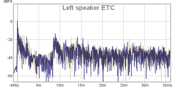
When the speakers were placed too close to the console, LEDR was sounding smeared and so were the phantom center tests. ETC curves were also showing some strong early (< 6 ms) reflections:

I moved the speakers further from the console and placed them wider, so they didn't get too close to the couch. Though, the right speaker was now too close to the right wall. Fortunately, the reflections from the wall can be defeated by rotating the speaker appropriately. The hint that I've read in the notes of S. Linkwitz was to put a mirror to the wall and ensure that from the listening position I see the speaker from the side. Since LXmini is a dipole speaker there is a null at the side, thus the most harmful reflection from the nearby wall is minimized. We can see that on the ETC graphs from the new position (the graphs from the initial position are blended in for comparison):

For the left speaker, instead of the two reflections above -20 dB within the first 6 ms there is now one of a bit lesser power. For the right speaker, the overall level of reflections arriving during the first 6 ms are significantly reduced, and its ETC graph resembles more the ETC of the left speaker.

Playing the test tracks has also confirmed the improvement—now I can feel the rattle sound in LEDR moving in vertical and front-back directions clearly. Also, by avoiding creating strong reflections for the right speaker, I've made it essentially equal to more "spacious" left speaker placement, thus the asymmetry of the listening space doesn't matter anymore. However, the resulting "aggressive" toeing in of the right speaker has narrowed the listening "sweet spot". Apparently, it's not easy to achieve a perfect setup under real life conditions.

Equalizing Speakers

From my previous measurements I knew that the quality of the speaker drivers used in LXminis make them well matched. However, my initial measurements has shown some discrepancy which I wanted to correct:

I'm not a fan of excessive equalization—I believe that our brains are a much more powerful computers than our audio analyzers. But adding a couple of filters to correct for speaker placement seems reasonable here. In this case, I reduced the amplitude of one of the notch filters in LXmini equalization and added a couple more filters:

Note that I didn't do anything below 50 Hz because I plan to use the subwoofer with the crossover frequency at 45 Hz.

Then I adjusted KRK 10s to inhibit its output in the range of 30–60 Hz to "boost" its output at 20 Hz. Here I used filters suggested by Room EQ Wizard for the listening position:

Subwoofer Alignment in Time Domain

This was the most challenging part. I connected subwoofer using a cascaded miniDSP 2x4 HD in the following way:

Additional processing delay, phase shifts, and asymmetric positioning together create a framework which is challenging to analyze. Instead, I decided to apply the approach suggested by the author of Acourate software Dr. Ulrich Brüggemann. The procedure consists of the following steps:

1. Capture the impulse response of the main speaker using Acourate without the subwoofer.
2. Capture the impulse response of high-passed main speaker plus the subwoofer. The high frequency part of the response allows Acourate to align these IRs in time.
3. Convolve both impulse responses with a sine wave from the overlapping region.
4. By comparing the mutual offsets of the resulting sine waves in the initial transient moment and during sustained period deduce time delay and possibly phase inversion.

As I've learned from my experience, aligning based on a single frequency in the Step 3 may not provide the best results as at low frequencies the phase and the group delay of speakers may fluctuate severely. So instead of using a single sine wave I used a log sweep range in the bass region. This doesn't provide data for aligning initial transients, but for bass frequencies I think the sustained stage is much more important.

Here is how convolutions with a log sweep from 40 to 100 Hz were looking initially for the left and right speaker:

The left graph is mostly aligned, while the right one shows a delay of the main speaker for 2.5 ms. It can be seen that even on the left speaker, the alignment in the low bass region is poorer than at higher frequencies. I don't consider that to be a problem because there the contribution of LXminis is negligible. It's much more important to time align the region where both the sub and the LXminis can be heard together. It's also easy to see that if we attempt to use the crossover frequency (45 Hz) as the anchor point for time alignment, the speakers would be out of phase for higher frequencies which will result in "sagged" frequency response.

To avoid compromising the alignment of the left speaker, I decided to delay the sub for 1.25 ms which improves alignment for the right speaker, but doesn't degrade it too much for the left one. Below are the graphs of LXminis filtered with Linkwitz-Riley 24 dB/oct crossover at 45 Hz and with added subwoofer:

Definitely we can see extended bass range. You can also feel it :) I think, setting the crossover point low allows to get the maximum fidelity from the LXminis + subwoofer combination.

With all this laborious setup done, it's time to enjoy music!